Backtracking is a general algorithm for finding all (or some) solutions to some computational problems (notably Constraint satisfaction problems or CSPs), which incrementally builds candidates to the solution and abandons a candidate (“backtracks”) as soon as it determines that the candidate cannot lead to a valid solution
Category: Utility
Recursion
Objectives
- Significance
- Flow of control
- Memory usage
- Interview FAQs
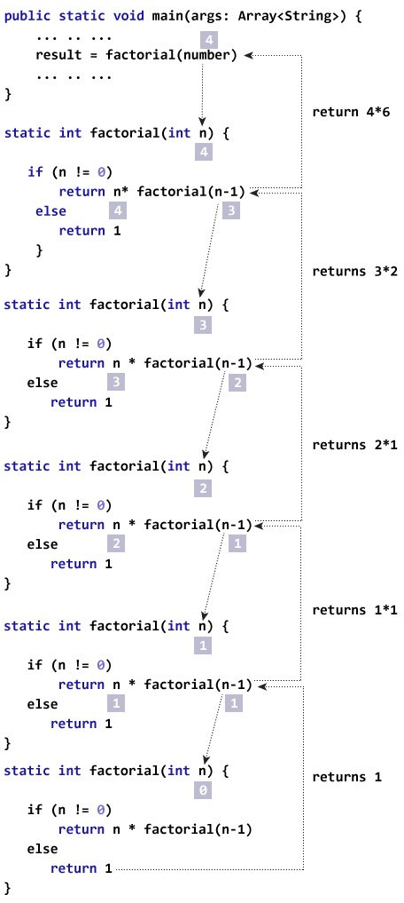
Recursion is a process by which a function or a method calls itself again and again. Analogy: Anything that can be done in for loop can be done by recursion
Iteration VS Recursion
| Criteria | Recursion | Iteration |
|---|---|---|
| Definition | Recursion is a process where a method calls itself repeatedly until a base condition is met. | Iteration is a process by which a piece of code is repeatedly executed for a finite number of times or until a condition is met. |
| Applicability | Is the application for functions. | Is applicable for loops. |
| Chunk of code can be applied to? | Works well for smaller code size. | Works well for larger code size. |
| Memory Footprint | Utilizes more memory as each recursive call is pushed to the stack | Comparatively less memory is used. |
| Maintainability | Difficult to debug and maintain | Easier to debug and maintain |
| Type of errors expected | Results in stack overflow if the base condition is not specified or not reached | May execute infinitely but will ultimately stop execution with any memory errors |
| Time-Complexity | Time complexity is very high. | Time complexity is relatively on the lower side. |
Structure : Any method that implements Recursion has two basic parts:
- Method call which can call itself i.e. recursive
- A precondition that will stop the recursion.
Note that a precondition is necessary for any recursive method as, if we do not break the recursion then it will keep on running infinitely and result in a stack overflow.
Syntax- The general syntax of recursion is as follows:
methodName (T parameters…)
{
    if (precondition == true)
//precondition or base condition
    {
        return result;
    }
    return methodName (T parameters…);

        //recursive call
}
Associated Error – Stack Overflow Error In Recursion
We are aware that when any method or function is called, the state of the function is stored on the stack and is retrieved when the function returns. The stack is used for the recursive method as well.
But in the case of recursion, a problem might occur if we do not define the base condition or when the base condition is somehow not reached or executed. If this situation occurs then the stack overflow may arise.
Types of recursion
- Tail Recursion
- Head Recursion
- Tree recursion
Tail Recursion
When the call to the recursive method is the last statement executed inside the recursive method, it is called “Tail Recursion”.
In tail recursion, the recursive call statement is usually executed along with the return statement of the method.
methodName ( T parameters…){
{
    if (base_condition == true)
    {
        return result;
    }
    return methodName (T parameters …)      //tail recursion
}
Head Recursion
Head recursion is any recursive approach that is not a tail recursion. So even general recursion is ahead recursion.
methodName (T parameters…){
    if (some_condition == true)
    {
        return methodName (T parameters…);
    }
    return result;
}
Tree Recursion
Has two recursive calls(Left/right sub-tree)
Problem-Solving Using Recursion
The basic idea behind using recursion is to express the bigger problem in terms of smaller problems. Also, we need to add one or more base conditions so that we can come out of recursion.
PAGE BREAK
FAQS
Q #1.How does Recursion work in Java?
Answer: In recursion, the recursive function calls itself repeatedly until a base condition is satisfied. The memory for the called function is pushed on to the stack at the top of the memory for the calling function. For each function call, a separate copy of local variables is made.
Q #2) Why is Recursion used?
Answer: Recursion is used to solve those problems that can be broken down into smaller ones and the entire problem can be expressed in terms of a smaller problem.
Recursion is also used for those problems that are too complex to be solved using an iterative approach. Besides the problems for which time complexity is not an issue, use recursion.
Q #3) What are the benefits of Recursion?
Answer:
The benefits of Recursion include:
- Recursion reduces redundant calling of function.
- Recursion allows us to solve problems easily when compared to the iterative approach.
Q #4) Which one is better – Recursion or Iteration?
Answer: Recursion makes repeated calls until the base function is reached. Thus there is a memory overhead as a memory for each function call is pushed on to the stack.
Iteration on the other hand does not have much memory overhead. Recursion execution is slower than the iterative approach. Recursion reduces the size of the code while the iterative approach makes the code large.
Recursion is better than the iterative approach for problems like the Tower of Hanoi, tree traversals, etc.
Question : how unflods while same method called:
https://leetcode.com/problems/merge-two-binary-trees/editorial/
Dynamic Programming
Index
- Introduction to Dynamic Programming
- Strategic Approach
- Common patterns
- Top-Down Approach – recursion+memorisation
- Bottom-up Approach – tabulation.
Introduction to Dynamic Programming
What is Dynamic Programming?
Dynamic Programming (DP) is a programming paradigm that can systematically and efficiently explore all possible solutions to a problem. As such, it is capable of solving a wide variety of problems that often have the following characteristics:
- The problem can be broken down into “overlapping subproblems” – smaller versions of the original problem that are re-used multiple times.
- The problem has an “optimal substructure” – an optimal solution can be formed from optimal solutions to the overlapping subproblems of the original problem.
Fibonacci Example –
If you wanted to find the n^{th}nth Fibonacci number F(n)F(n), you can break it down into smaller subproblems – find F(n – 1)F(n−1) and F(n – 2)F(n−2) instead. Then, adding the solutions to these subproblems together gives the answer to the original question, F(n – 1) + F(n – 2) = F(n)F(n−1)+F(n−2)=F(n), which means the problem has optimal substructure, since a solution F(n)F(n) to the original problem can be formed from the solutions to the subproblems. These subproblems are also overlapping – for example, we would need F(4)F(4) to calculate both F(5)F(5) and F(6)F(6).
These attributes may seem familiar to you. Greedy problems have optimal substructure, but not overlapping subproblems. Divide and conquer algorithms break a problem into subproblems, but these subproblems are not overlapping (which is why DP and divide and conquer are commonly mistaken for one another).
There are two ways to implement a DP algorithm:
- Bottom-up, also known as tabulation.
- Top-down, also known as memoization.
Bottom-up (Tabulation)
Bottom-up is implemented with iteration and starts at the base cases. Let’s use the Fibonacci sequence as an example again. The base cases for the Fibonacci sequence are F(0)=0 and F(1) = 1. With bottom-up, we would use these base cases to calculate F(2)F(2), and then use that result to calculate F(3), and so on all the way up to F(n)
Pseudi COde
// Pseudocode example for bottom-up

F = array of length (n + 1)
F[0] = 0
F[1] = 1
for i from 2 to n:
    F[i] = F[i - 1] + F[i - 2]
Top-down (Memoization)

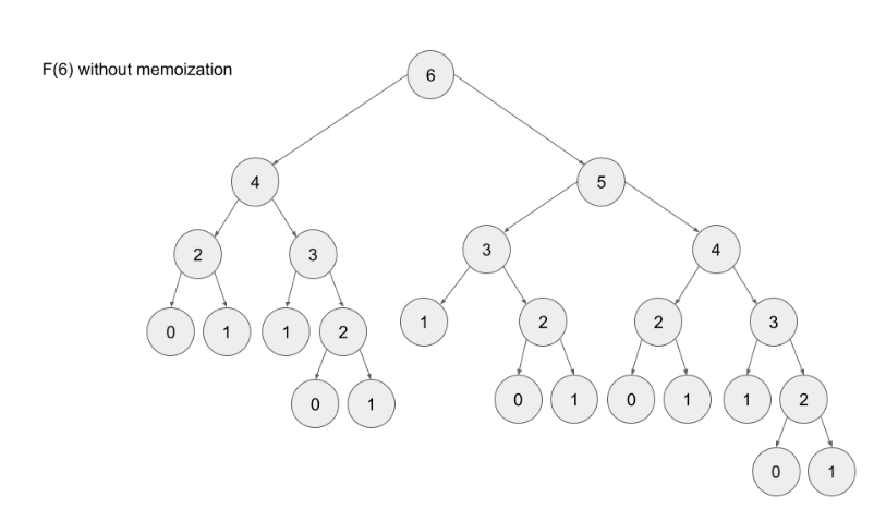
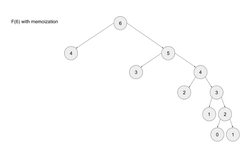
Top-down is implemented with recursion and made efficient with memoization. If we wanted to find the n^{th}nth Fibonacci number F(n)F(n), we try to compute this by finding F(n – 1)F(n−1) and F(n – 2)F(n−2). This defines a recursive pattern that will continue on until we reach the base cases F(0) = F(1) = 1F(0)=F(1)=1. The problem with just implementing it recursively is that there is a ton of unnecessary repeated computation. Take a look at the recursion tree if we were to find F(5)F(5):

Notice that we need to calculate F(2) three times. This might not seem like a big deal, but if we were to calculate F(6), this entire image would be only one child of the root. Imagine if we wanted to find F(100) – the amount of computation is exponential and will quickly explode. The solution to this is to memoize results.
Note- memoizing a result means to store the result of a function call, usually in a hashmap or an array, so that when the same function call is made again, we can simply return the memoized result instead of recalculating the result.
Advantages
- It is very easy to understand and implement.
- It solves the subproblems only when it is required.
- It is easy to debug.
Disadvantages
- It uses the recursion technique that occupies more memory in the call stack.
- Sometimes when the recursion is too deep, the stack overflow condition will occur.
- It occupies more memory that degrades the overall performance.
When to Use DP
Following are the scenarios to use DP-
- The problem can be broken down into “overlapping subproblems” – smaller versions of the original problem that are re-used multiple times
- The problem has an “optimal substructure” – an optimal solution can be formed from optimal solutions to the overlapping subproblems of the original problem.
Unfortunately, it is hard to identify when a problem fits into these definitions. Instead, let’s discuss some common characteristics of DP problems that are easy to identify.
The first characteristic that is common in DP problems is that the problem will ask for the optimum value (maximum or minimum) of something, or the number of ways there are to do something. For example:
- Optimization problems.
- What is the minimum cost of doing…
- What is the maximum profit from…
- How many ways are there to do…
- What is the longest possible…
- Is it possible to reach a certain point…
- Combinatorial problems.
- given a number N, you’ve to find the number of different ways to write it as the sum of 1, 3 and 4.
Note: Not all DP problems follow this format, and not all problems that follow these formats should be solved using DP. However, these formats are very common for DP problems and are generally a hint that you should consider using dynamic programming.
When it comes to identifying if a problem should be solved with DP, this first characteristic is not sufficient. Sometimes, a problem in this format (asking for the max/min/longest etc.) is meant to be solved with a greedy algorithm. The next characteristic will help us determine whether a problem should be solved using a greedy algorithm or dynamic programming.
The second characteristic that is common in DP problems is that future “decisions” depend on earlier decisions. Deciding to do something at one step may affect the ability to do something in a later step. This characteristic is what makes a greedy algorithm invalid for a DP problem – we need to factor in results from previous decisions.
Algorithm –
You can either use Map or array to store/memoize the elements (both gives O(1) access time.
Utilities :
Utilities
- Glimpse
- Code Template
- Two pointers
- Sliding window
- LinkedLIst
- Tree
- Graph
- Heap
- Binary search
- BackTracking
- Dynamic programming
- Dijkstra Algorithm
- Quick Notes – Cheatsheet
- Code Template
- Utilities
- Occurrence-count
- Using additional DS i.e Map
- Without using additional DS
- Character
- Convert character to upper case
- Matrix Properties
- Probable ArrayIndexOutOfBound
- Graceful handling
- Taking input-Bugfree in java
- Occurrence-count
Code Template
Here are code templates for common patterns for all the data structures and algorithms:
Two pointers: one input, opposite ends
public int fn(int[] arr) {
    int left = 0;
    int right = arr.length - 1;
    int ans = 0;

    while (left < right) {
        // do some logic here with left and right
        if (CONDITION) {
            left++;
        } else {
            right--;
        }
    }

    return ans;
}
Two pointers: two inputs, exhaust both
public int fn(int[] arr1, int[] arr2) {
    int i = 0, j = 0, ans = 0;

    while (i < arr1.length && j < arr2.length) {
        // do some logic here
        if (CONDITION) {
            i++;
        } else {
            j++;
        }
    }

    while (i < arr1.length) {
        // do logic
        i++;
    }

    while (j < arr2.length) {
        // do logic
        j++;
    }

    return ans;
}
Sliding window
public int fn(int[] arr) {
    int left = 0, ans = 0, curr = 0;

    for (int curr = 0; curr < arr.length; curr++) {
        // do logic here to add arr[right] to curr

        while (WINDOW_CONDITION_BROKEN) {
            // remove arr[left] from curr
            left++;
        }

        // update ans
    }

    return ans;
}
Build a prefix sum (left sum)
public int[] fn(int[] arr) {
    int[] prefix = new int[arr.length];
    prefix[0] = arr[0];

    for (int i = 1; i < arr.length; i++) {
        prefix[i] = prefix[i - 1] + arr[i];
    }

    return prefix;
}
Efficient string building
public String fn(char[] arr) {
    StringBuilder sb = new StringBuilder();
    for (char c: arr) {
        sb.append(c);
    }

    return sb.toString();
}
Linked list: fast and slow pointer
public int fn(ListNode head) {
    ListNode slow = head;
    ListNode fast = head;
    int ans = 0;

    while (fast != null && fast.next != null) {
        // do logic
        slow = slow.next;
        fast = fast.next.next;
    }

    return ans;
}
Find number of subarrays that fit an exact criteria
//TOdo - what purpose
public int fn(int[] arr, int k) {
    Map<Integer, Integer> counts = new HashMap<>();
    counts.put(0, 1);
    int ans = 0, curr = 0;

    for (int num: arr) {
        // do logic to change curr
        ans += counts.getOrDefault(curr - k, 0);
        counts.put(curr, counts.getOrDefault(curr, 0) + 1);
    }

    return ans;
}
Monotonic increasing stack
//The same logic can be applied to maintain a monotonic queue.
public int fn(int[] arr) {
    Stack<Integer> stack = new Stack<>();
    int ans = 0;

    for (int num: arr) {
        // for monotonic decreasing, just flip the > to <
        while (!stack.empty() && stack.peek() > num) {
            // do logic
            stack.pop();
        }

        stack.push(num);
    }

    return ans;
}
Binary tree: DFS (recursive)
public int dfs(TreeNode root) {
    if (root == null) {
        return 0;
    }

    int ans = 0;
    // do logic
    dfs(root.left);
    dfs(root.right);
    return ans;
}
Binary tree: DFS (iterative)
public int dfs(TreeNode root) {
    Stack<TreeNode> stack = new Stack<>();
    stack.push(root);
    int ans = 0;

    while (!stack.empty()) {
        TreeNode node = stack.pop();
        // do logic
        if (node.left != null) {
            stack.push(node.left);
        }
        if (node.right != null) {
            stack.push(node.right);
        }
    }

    return ans;
}
Binary tree: BFS
public int fn(TreeNode root) {
    Queue<TreeNode> queue = new LinkedList<>();
    queue.add(root);
    int ans = 0;

    while (!queue.isEmpty()) {
        int currentLength = queue.size();
        // do logic for current level

        for (int i = 0; i < currentLength; i++) {
            TreeNode node = queue.remove();
            // do logic
            if (node.left != null) {
                queue.add(node.left);
            }
            if (node.right != null) {
                queue.add(node.right);
            }
        }
    }

    return ans;
}
Graph: DFS (recursive)
For the graph templates, assume the nodes are numbered from 0 to n - 1 and the graph is given as an adjacency list. Depending on the problem, you may need to convert the input into an equivalent adjacency list before using the templates.
Set<Integer> seen = new HashSet<>();

public int fn(int[][] graph) {
    seen.add(START_NODE);
    return dfs(START_NODE, graph);
}

public int dfs(int node, int[][] graph) {
    int ans = 0;
    // do some logic
    for (int neighbor: graph[node]) {
        if (!seen.contains(neighbor)) {
            seen.add(neighbor);
            ans += dfs(neighbor, graph);
        }
    }

    return ans;
}
Graph: DFS (iterative)
public int fn(int[][] graph) {
    Stack<Integer> stack = new Stack<>();
    Set<Integer> seen = new HashSet<>();
    stack.push(START_NODE);
    seen.add(START_NODE);
    int ans = 0;

    while (!stack.empty()) {
        int node = stack.pop();
        // do some logic
        for (int neighbor: graph[node]) {
            if (!seen.contains(neighbor)) {
                seen.add(neighbor);
                stack.push(neighbor);
            }
        }
    }

    return ans;
}
Graph: BFS
public int fn(int[][] graph) {
    Queue<Integer> queue = new LinkedList<>();
    Set<Integer> seen = new HashSet<>();
    queue.add(START_NODE);
    seen.add(START_NODE);
    int ans = 0;

    while (!queue.isEmpty()) {
        int node = queue.remove();
        // do some logic
        for (int neighbor: graph[node]) {
            if (!seen.contains(neighbor)) {
                seen.add(neighbor);
                queue.add(neighbor);
            }
        }
    }

    return ans;
}
Find top k elements with heap
public int[] fn(int[] arr, int k) {
    PriorityQueue<Integer> heap = new PriorityQueue<>(CRITERIA);
    for (int num: arr) {
        heap.add(num);
        if (heap.size() > k) {
            heap.remove();
        }
    }

    int[] ans = new int[k];
    for (int i = 0; i < k; i++) {
        ans[i] = heap.remove();
    }

    return ans;
}
Binary search
public int fn(int[] arr, int target) {
    int left = 0;
    int right = arr.length - 1;
    while (left <= right) {
        int mid = left + (right - left) / 2;
        if (arr[mid] == target) {
            // do something
            return mid;
        }
        if (arr[mid] > target) {
            right = mid - 1;
        } else {
            left = mid + 1;
        }
    }

    // left is the insertion point
    return left;
}
Binary search: duplicate elements, left-most insertion point
public int fn(int[] arr, int target) {
    int left = 0;
    int right = arr.length;
    while (left < right) {
        int mid = left + (right - left) / 2;
        if (arr[mid] >= target) {
            right = mid;
        } else {
            left = mid + 1;
        }
    }

    return left;
}
Binary search: duplicate elements, right-most insertion point
public int fn(int[] arr, int target) {
    int left = 0;
    int right = arr.length;
    while (left < right) {
        int mid = left + (right - left) / 2;
        if (arr[mid] > target) {
            right = mid;
        } else {
            left = mid + 1;
        }
    }

    return left;
}
Binary search: for greedy problems
If looking for a minimum:
public int fn(int[] arr) {
    int left = MINIMUM_POSSIBLE_ANSWER;
    int right = MAXIMUM_POSSIBLE_ANSWER;
    while (left <= right) {
        int mid = left + (right - left) / 2;
        if (check(mid)) {
            right = mid - 1;
        } else {
            left = mid + 1;
        }
    }

    return left;
}

public boolean check(int x) {
    // this function is implemented depending on the problem
    return BOOLEAN;
}
If looking for a maximum:
public int fn(int[] arr) {
    int left = MINIMUM_POSSIBLE_ANSWER;
    int right = MAXIMUM_POSSIBLE_ANSWER;
    while (left <= right) {
        int mid = left + (right - left) / 2;
        if (check(mid)) {
            left = mid + 1;
        } else {
            right = mid - 1;
        }
    }

    return right;
}

public boolean check(int x) {
    // this function is implemented depending on the problem
    return BOOLEAN;
}
Backtracking
public int backtrack(STATE curr, OTHER_ARGUMENTS...) {
    if (BASE_CASE) {
        // modify the answer
        return 0;
    }

    int ans = 0;
    for (ITERATE_OVER_INPUT) {
        // modify the current state
        ans += backtrack(curr, OTHER_ARGUMENTS...)
        // undo the modification of the current state
    }
}
Dynamic programming: top-down memoization
Map<STATE, Integer> memo = new HashMap<>();

public int fn(int[] arr) {
    return dp(STATE_FOR_WHOLE_INPUT, arr);
}

public int dp(STATE, int[] arr) {
    if (BASE_CASE) {
        return 0;
    }

    if (memo.contains(STATE)) {
        return memo.get(STATE);
    }

    int ans = RECURRENCE_RELATION(STATE);
    memo.put(STATE, ans);
    return ans;
}
Build a trie
// note: using a class is only necessary if you want to store data at each node.
// otherwise, you can implement a trie using only hash maps.
class TrieNode {
    // you can store data at nodes if you wish
    int data;
    Map<Character, TrieNode> children;
    TrieNode() {
        this.children = new HashMap<>();
    }
}

public TrieNode buildTrie(String[] words) {
    TrieNode root = new TrieNode();
    for (String word: words) {
        TrieNode curr = root;
        for (char c: word.toCharArray()) {
            if (!curr.children.containsKey(c)) {
                curr.children.put(c, new TrieNode());
            }

            curr = curr.children.get(c);
        }

        // at this point, you have a full word at curr
        // you can perform more logic here to give curr an attribute if you want
    }

    return root;
}
Dijkstra’s algorithm
int[] distances = new int[n];
Arrays.fill(distances, Integer.MAX_VALUE);
distances[source] = 0;

Queue<Pair<Integer, Integer>> heap = new PriorityQueue<Pair<Integer,Integer>>(Comparator.comparing(Pair::getKey));
heap.add(new Pair(0, source));

while (!heap.isEmpty()) {
    Pair<Integer, Integer> curr = heap.remove();
    int currDist = curr.getKey();
    int node = curr.getValue();

    if (currDist > distances[node]) {
        continue;
    }

    for (Pair<Integer, Integer> edge: graph.get(node)) {
        int nei = edge.getKey();
        int weight = edge.getValue();
        int dist = currDist + weight;

        if (dist < distances[nei]) {
            distances[nei] = dist;
            heap.add(new Pair(dist, nei));
        }
    }
}
Quick Notes – Cheat-sheet
This article will be a collection of cheat sheets that you can use as you solve problems and prepare for interviews. You will find:
- Time complexity (Big O) cheat sheet
- General DS/A flowchart (when to use each DS/A)
- Stages of an interview cheat sheet
Time complexity (Big O) cheat sheet

First, let’s talk about the time complexity of common operations, split by data structure/algorithm. Then, we’ll talk about reasonable complexities given input sizes.
Arrays (dynamic array/list)
Given n = arr.length,
- Add or remove element at the end: �(1)O(1) amortized
- Add or remove element from arbitrary index: �(�)O(n)
- Access or modify element at arbitrary index: �(1)O(1)
- Check if element exists: �(�)O(n)
- Two pointers: �(�⋅�)O(n⋅k), where �k is the work done at each iteration, includes sliding window
- Building a prefix sum: �(�)O(n)
- Finding the sum of a subarray given a prefix sum: �(1)O(1)
Strings (immutable)
Given n = s.length,
- Add or remove character: �(�)O(n)
- Access element at arbitrary index: �(1)O(1)
- Concatenation between two strings: �(�+�)O(n+m), where �m is the length of the other string
- Create substring: �(�)O(m), where �m is the length of the substring
- Two pointers: �(�⋅�)O(n⋅k), where �k is the work done at each iteration, includes sliding window
- Building a string from joining an array, stringbuilder, etc.: �(�)O(n)
Linked Lists
Given �n as the number of nodes in the linked list,
- Add or remove element given pointer before add/removal location: �(1)O(1)
- Add or remove element given pointer at add/removal location: �(1)O(1) if doubly linked
- Add or remove element at arbitrary position without pointer: �(�)O(n)
- Access element at arbitrary position without pointer: �(�)O(n)
- Check if element exists: �(�)O(n)
- Reverse between position
iandj: �(�−�)O(j−i) - Detect a cycle: �(�)O(n) using fast-slow pointers or hash map
Hash table/dictionary
Given n = dic.length,
- Add or remove key-value pair: �(1)O(1)
- Check if key exists: �(1)O(1)
- Check if value exists: �(�)O(n)
- Access or modify value associated with key: �(1)O(1)
- Iterate over all keys, values, or both: �(�)O(n)
Note: the �(1)O(1) operations are constant relative to
n. In reality, the hashing algorithm might be expensive. For example, if your keys are strings, then it will cost �(�)O(m) where �m is the length of the string. The operations only take constant time relative to the size of the hash map.
Set
Given n = set.length,
- Add or remove element: �(1)O(1)
- Check if element exists: �(1)O(1)
The above note applies here as well.
Stack
Stack operations are dependent on their implementation. A stack is only required to support pop and push. If implemented with a dynamic array:
Given n = stack.length,
- Push element: �(1)O(1)
- Pop element: �(1)O(1)
- Peek (see element at top of stack): �(1)O(1)
- Access or modify element at arbitrary index: �(1)O(1)
- Check if element exists: �(�)O(n)
Queue
Queue operations are dependent on their implementation. A queue is only required to support dequeue and enqueue. If implemented with a doubly linked list:
Given n = queue.length,
- Enqueue element: �(1)O(1)
- Dequeue element: �(1)O(1)
- Peek (see element at front of queue): �(1)O(1)
- Access or modify element at arbitrary index: �(�)O(n)
- Check if element exists: �(�)O(n)
Note: most programming languages implement queues in a more sophisticated manner than a simple doubly linked list. Depending on implementation, accessing elements by index may be faster than �(�)O(n), or �(�)O(n) but with a significant constant divisor.
Binary tree problems (DFS/BFS)
Given �n as the number of nodes in the tree,
Most algorithms will run in �(�⋅�)O(n⋅k) time, where �k is the work done at each node, usually �(1)O(1). This is just a general rule and not always the case. We are assuming here that BFS is implemented with an efficient queue.
Binary search tree
Given �n as the number of nodes in the tree,
- Add or remove element: �(�)O(n) worst case, �(log�)O(logn) average case
- Check if element exists: �(�)O(n) worst case, �(log�)O(logn) average case
The average case is when the tree is well balanced – each depth is close to full. The worst case is when the tree is just a straight line.
Heap/Priority Queue
Given n = heap.length and talking about min heaps,
- Add an element: �(log�)O(logn)
- Delete the minimum element: �(log�)O(logn)
- Find the minimum element: �(1)O(1)
- Check if element exists: �(�)O(n)
Binary search
Binary search runs in �(log�)O(logn) in the worst case, where �n is the size of your initial search space.
Miscellaneous
- Sorting: �(�⋅log�)O(n⋅logn), where �n is the size of the data being sorted
- DFS and BFS on a graph: �(�⋅�+�)O(n⋅k+e), where �n is the number of nodes, �e is the number of edges, if each node is handled in �(1)O(1) other than iterating over edges
- DFS and BFS space complexity: typically �(�)O(n), but if it’s in a graph, might be �(�+�)O(n+e) to store the graph
- Dynamic programming time complexity: �(�⋅�)O(n⋅k), where �n is the number of states and �k is the work done at each state
- Dynamic programming space complexity: �(�)O(n), where �n is the number of states
Input sizes vs time complexity
The constraints of a problem can be considered as hints because they indicate an upper bound on what your solution’s time complexity should be. Being able to figure out the expected time complexity of a solution given the input size is a valuable skill to have. In all LeetCode problems and most online assessments (OA), you will be given the problem’s constraints. Unfortunately, you will usually not be explicitly told the constraints of a problem in an interview, but it’s still good for practicing on LeetCode and completing OAs. Still, in an interview, it usually doesn’t hurt to ask about the expected input sizes.
n <= 10
The expected time complexity likely has a factorial or an exponential with a base larger than 2 – �(�2⋅�!)O(n2⋅n!) or �(4�)O(4n) for example.
You should think about backtracking or any brute-force-esque recursive algorithm. n <= 10 is extremely small and usually any algorithm that correctly finds the answer will be fast enough.
10 < n <= 20
The expected time complexity likely involves �(2�)O(2n). Any higher base or a factorial will be too slow (320320 = ~3.5 billion, and 20!20! is much larger). A 2�2n usually implies that given a collection of elements, you are considering all subsets/subsequences – for each element, there are two choices: take it or don’t take it.
Again, this bound is very small, so most algorithms that are correct will probably be fast enough. Consider backtracking and recursion.
20 < n <= 100
At this point, exponentials will be too slow. The upper bound will likely involve �(�3)O(n3).
Problems marked as “easy” on LeetCode usually have this bound, which can be deceiving. There may be solutions that run in �(�)O(n), but the small bound allows brute force solutions to pass (finding the linear time solution might not be considered as “easy”).
Consider brute force solutions that involve nested loops. If you come up with a brute force solution, try analyzing the algorithm to find what steps are “slow”, and try to improve on those steps using tools like hash maps or heaps.
100 < n <= 1,000
In this range, a quadratic time complexity �(�2)O(n2) should be sufficient, as long as the constant factor isn’t too large.
Similar to the previous range, you should consider nested loops. The difference between this range and the previous one is that �(�2)O(n2) is usually the expected/optimal time complexity in this range, and it might not be possible to improve.
1,000 < n < 100,000
�<=105n<=105 is the most common constraint you will see on LeetCode. In this range, the slowest acceptable common time complexity is �(�⋅log�)O(n⋅logn), although a linear time approach �(�)O(n) is commonly the goal.
In this range, ask yourself if sorting the input or using a heap can be helpful. If not, then aim for an �(�)O(n) algorithm. Nested loops that run in �(�2)O(n2) are unacceptable – you will probably need to make use of a technique learned in this course to simulate a nested loop’s behavior in �(1)O(1) or �(log�)O(logn):
- Hash map
- A two pointers implementation like sliding window
- Monotonic stack
- Binary search
- Heap
- A combination of any of the above
If you have an �(�)O(n) algorithm, the constant factor can be reasonably large (around 40). One common theme for string problems involves looping over the characters of the alphabet at each iteration resulting in a time complexity of �(26�)O(26n).
100,000 < n < 1,000,000
�<=106n<=106 is a rare constraint, and will likely require a time complexity of �(�)O(n). In this range, �(�⋅log�)O(n⋅logn) is usually safe as long as it has a small constant factor. You will very likely need to incorporate a hash map in some way.
1,000,000 < n
With huge inputs, typically in the range of 109109 or more, the most common acceptable time complexity will be logarithmic �(log�)O(logn) or constant �(1)O(1). In these problems, you must either significantly reduce your search space at each iteration (usually binary search) or use clever tricks to find information in constant time (like with math or a clever use of hash maps).
Other time complexities are possible like �(�)O(n), but this is very rare and will usually only be seen in very advanced problems.
Sorting algorithms
All major programming languages have a built-in method for sorting. It is usually correct to assume and say sorting costs �(�⋅log�)O(n⋅logn), where �n is the number of elements being sorted. For completeness, here is a chart that lists many common sorting algorithms and their completeness. The algorithm implemented by a programming language varies; for example, Python uses Timsort but in C++, the specific algorithm is not mandated and varies.

Definition of a stable sort from Wikipedia: “Stable sorting algorithms maintain the relative order of records with equal keys (i.e. values). That is, a sorting algorithm is stable if whenever there are two records R and S with the same key and with R appearing before S in the original list, R will appear before S in the sorted list.”
General DS/A flowchart
Here’s a flowchart that can help you figure out which data structure or algorithm should be used. Note that this flowchart is very general as it would be impossible to cover every single scenario.
Note that this flowchart only covers methods taught in LICC, and as such more advanced algorithms like Dijkstra’s is excluded.

