Dynamic Programming (DP) is a programming paradigm that can systematically and efficiently explore all possible solutions to a problem. As such, it is capable of solving a wide variety of problems that often have the following characteristics:
The problem can be broken down into “overlapping subproblems” – smaller versions of the original problem that are re-used multiple times.
The problem has an “optimal substructure” – an optimal solution can be formed from optimal solutions to the overlapping subproblems of the original problem.
Fibonacci Example –
If you wanted to find the n^{th}nth Fibonacci number F(n)F(n), you can break it down into smaller subproblems – find F(n – 1)F(n−1) and F(n – 2)F(n−2) instead. Then, adding the solutions to these subproblems together gives the answer to the original question, F(n – 1) + F(n – 2) = F(n)F(n−1)+F(n−2)=F(n), which means the problem has optimal substructure, since a solution F(n)F(n) to the original problem can be formed from the solutions to the subproblems. These subproblems are also overlapping – for example, we would need F(4)F(4) to calculate both F(5)F(5) and F(6)F(6).
These attributes may seem familiar to you. Greedy problems have optimal substructure, but not overlapping subproblems. Divide and conquer algorithms break a problem into subproblems, but these subproblems are not overlapping (which is why DP and divide and conquer are commonly mistaken for one another).
There are two ways to implement a DP algorithm:
Bottom-up, also known as tabulation.
Top-down, also known as memoization.
Bottom-up (Tabulation)
Bottom-up is implemented with iteration and starts at the base cases. Let’s use the Fibonacci sequence as an example again. The base cases for the Fibonacci sequence are F(0)=0 and F(1) = 1. With bottom-up, we would use these base cases to calculate F(2)F(2), and then use that result to calculate F(3), and so on all the way up to F(n)
Pseudi COde
// Pseudocode example for bottom-up

F = array of length (n + 1)
F[0] = 0
F[1] = 1
for i from 2 to n:
    F[i] = F[i - 1] + F[i - 2]
Top-down (Memoization)
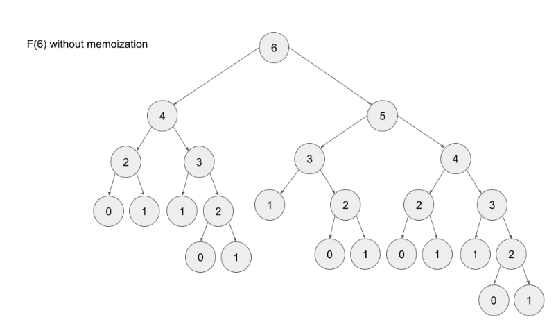
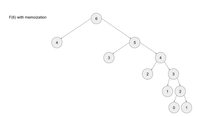
Top-down is implemented with recursion and made efficient with memoization. If we wanted to find the n^{th}nth Fibonacci number F(n)F(n), we try to compute this by finding F(n – 1)F(n−1) and F(n – 2)F(n−2). This defines a recursive pattern that will continue on until we reach the base cases F(0) = F(1) = 1F(0)=F(1)=1. The problem with just implementing it recursively is that there is a ton of unnecessary repeated computation. Take a look at the recursion tree if we were to find F(5)F(5):
Notice that we need to calculate F(2) three times. This might not seem like a big deal, but if we were to calculate F(6), this entire image would be only one child of the root. Imagine if we wanted to find F(100) – the amount of computation is exponential and will quickly explode. The solution to this is to memoize results.
Note- memoizing a result means to store the result of a function call, usually in a hashmap or an array, so that when the same function call is made again, we can simply return the memoized result instead of recalculating the result.
memorisation vs without memorisation
Advantages
It is very easy to understand and implement.
It solves the subproblems only when it is required.
It is easy to debug.
Disadvantages
It uses the recursion technique that occupies more memory in the call stack.
Sometimes when the recursion is too deep, the stack overflow condition will occur.
It occupies more memory that degrades the overall performance.
When to Use DP
Following are the scenarios to use DP-
The problem can be broken down into “overlapping subproblems” – smaller versions of the original problem that are re-used multiple times
The problem has an “optimal substructure” – an optimal solution can be formed from optimal solutions to the overlapping subproblems of the original problem.
Unfortunately, it is hard to identify when a problem fits into these definitions. Instead, let’s discuss some common characteristics of DP problems that are easy to identify.
The first characteristic that is common in DP problems is that the problem will ask for the optimum value (maximum or minimum) of something, or the number of ways there are to do something. For example:
Optimization problems.
What is the minimum cost of doing…
What is the maximum profit from…
How many ways are there to do…
What is the longest possible…
Is it possible to reach a certain point…
Combinatorial problems.
given a number N, you’ve to find the number of different ways to write it as the sum of 1, 3 and 4.
Note: Not all DP problems follow this format, and not all problems that follow these formats should be solved using DP. However, these formats are very common for DP problems and are generally a hint that you should consider using dynamic programming.
When it comes to identifying if a problem should be solved with DP, this first characteristic is not sufficient. Sometimes, a problem in this format (asking for the max/min/longest etc.) is meant to be solved with a greedy algorithm. The next characteristic will help us determine whether a problem should be solved using a greedy algorithm or dynamic programming.
The second characteristic that is common in DP problems is that future “decisions” depend on earlier decisions. Deciding to do something at one step may affect the ability to do something in a later step. This characteristic is what makes a greedy algorithm invalid for a DP problem – we need to factor in results from previous decisions.
Algorithm –
You can either use Map or array to store/memoize the elements (both gives O(1) access time.
Inserting node (tc -O(n) -if emenents are skewed one sided (left/right)-need to traversed the all nodes i.e height of tree to insert)
Searching for a node (tc -O(n))
Questions
Tree Implementation
Node representation
Inserting node in BST
Tree-traversal
DFS
Recursively (hard to explain in case of backtracking)
Iteratively (using stack)
Questions
BFS
Iteratively (using queue)
Questions
Expression tree & Binary Tree
Topics Covered-
Definition & Components of tree
Where to use?
Denoting Tree in Java
Types of Tree
Traversal and searching
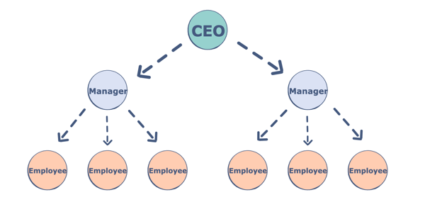
Trees are non-linear data structures. They are often used to represent hierarchical data. For a real-world example, a hierarchical company structure uses a tree to organize.
Tree have 1:N parent-child relation, if N is 2 then we call it Binary Tree
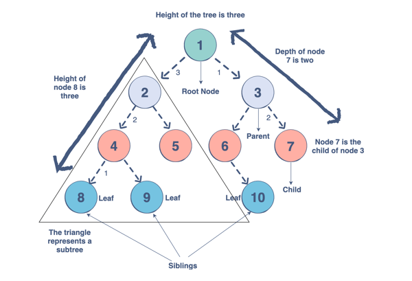
Components of a Tree
Trees are a collection of nodes (vertices), and they are linked with edges (pointers), representing the hierarchical connections between the nodes. A node contains data of any type, but all the nodes must be of the same data type. Trees are similar to graphs, but a cycle cannot exist in a tree. What are the different components of a tree?
Root: The root of a tree is a node that has no incoming link (i.e. no parent node). Think of this as a starting point of your tree.
Children: The child of a tree is a node with one incoming link from a node above it (i.e. a parent node). If two children nodes share the same parent, they are called siblings.
Parent: The parent node has an outgoing link connecting it to one or more child nodes
Leaf: A leaf has a parent node but has no outgoing link to a child node. Think of this as an endpoint of your tree.
Subtree: A subtree is a smaller tree held within a larger tree. The root of that tree can be any node from the bigger tree.
Depth: The depth of a node is the number of edges between that node and the root. Think of this as how many steps there are between your node and the tree’s starting point.
Height: The height of a node is the number of edges in the longest path from a node to a leaf node. Think of this as how many steps there are between your node and the tree’s endpoint. The height of a tree is the height of its root node.
Degree: The degree of a node refers to the number of sub-trees.
Why do we use trees?
The hierarchical structure gives a tree unique properties for storing, manipulating, and accessing data.We can use a tree for the following:
Storage as hierarchy. Storing information that naturally occurs in a hierarchy. File systems on a computer and PDF use tree structures.
Searching. Storing information that we want to search quickly. Trees are easier to search than a Linked List. Some types of trees (like AVL and Red-Black trees) are designed for fast searching.
Inheritance. Trees are used for inheritance, XML parser, machine learning, and DNS, amongst many other things.
Indexing. Advanced types of trees, like B-Trees and B+ Trees, can be used for indexing a database.
Networking. Trees are ideal for things like social networking and computer chess games.
Shortest path. A Spanning Tree can be used to find the shortest paths in routers for networking.
How to make a tree/?
To build a tree in Java we start with the root node.
Node<String> root = new Node<>("root");
Once we have our root, we can add our first child node using addChild, which adds a child node and assigns it to a parent node. We refer to this process as insertion (adding nodes) and deletion (removing nodes)
There are many types of trees that we can use to organize data differently within a hierarchical structure.The tree we use depends on the problem we are trying to solve. Let’s take a look at the trees we can use in Java. We will be covering:
N-ary trees
Balanced trees
Binary trees
Binary Search Trees
AVL Trees
Red-Black Trees
2-3 Trees
2-3-4 Trees
There are 3 main types of Binary tree based on thier structureL
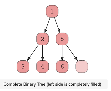
1.Complete Binary Tree
A complete binary tree exists when every level, excluding the last, is filled and all nodes at the last level are as far left as they can be. Here is a visual representation of a complete binary tree.
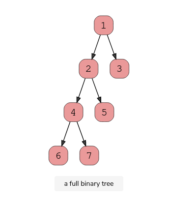
2.Full Binary Tree
A full binary tree (sometimes called proper binary tree) exits when every node, excluding the leaves, has two children. Every level must be filled, and the nodes are as far left as possible. Look at this diagram to understand how a full binary tree looks.
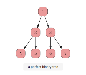
3.Perfect Binary Tree
A perfect binary tree should be both full and complete. All interior nodes should have two children, and all leaves must have the same depth. Look at this diagram to understand how a perfect binary tree looks.
A perfect binary tree should be both full and complete. All interior nodes should have two children, and all leaves must have the same depth. Look at this diagram to understand how a perfect binary tree looks.
Binary Search Trees
A Binary Search Tree is a binary tree in which every node has a key and an associated value. This allows for quick lookup and edits (additions or removals), hence the name “search”.
It’s important to note that every Binary Search Tree is a binary tree, but not every binary tree is a Binary Search Tree.
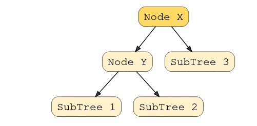
What makes them different? In a Binary Search Tree, the left subtree of a subtree must contain nodes with fewer(smaller) keys than a node’s key, while the right subtree will contain nodes with keys greater than that node’s key. Take a look at this visual to understand this condition.
In this example, the node Y is a parent node with two child nodes. All nodes in subtree 1 must have a value less than node Y, and subtree 2 must have a greater value than node Y.
Red Black Tree (Used in HashMap Java-8)
Intro to Tree Traversal and Searching
To use trees, we can traverse them by visiting/checking every node of a tree. If a tree is “traversed”, this means every node has been visited. There are four ways to traverse a tree. These four processes fall into one of two categories: breadth-first traversal or depth-first traversal.
Note : the traversal technique – in-order, pre-order and post-order only applies to binary tree where as DFS (iteratively using stack)can also be used for general graph for traversal.
DFS 3 OPTIONS (Position of root node)-
In-order ,
post-order (for deleting nodes),
preorder (preorder expression)
BFS – one- option
Level order
In-order Traversal –
as the name suggests gives the sorted number [in ascending order]
Think of this as moving up the tree, then back down. You traverse the left child and its sub-tree until you reach the root. Then, traverse down the right child and its subtree. This is a depth-first traversal.
Manual traversal hind- take the traversal order (LrR)–>1st one to print is L sub-tree(take the L sub tree as a tree and apply LrR)
Pre-order Traversal –
Helps in creating the copy of the tree.Preorder traversal is also used to get prefix expression on of an expression tree.
This of this as starting at the top, moving down, and then over. You start at the root, traverse the left sub-tree, and then move over to the right sub-tree. This is a depth-first traversal.
Manual traversal hind- take the traversal order (rLR)–>1st one to print is L sub-tree(take the L sub tree as a tree and apply rLR)
Post-order Traversal –
Aids in deletion of nodes as it traverses the child nodes first and then the root node..so helps avoid orphan node while deleting nodes .Postorder traversal is also useful to get the postfix expression of an expression tree.
Begin with the left-sub tree and move over to the right sub-tree. Then, move up to visit the root node. This is a depth-first traversal
Levelorder: Think of this as a sort of zig-zag pattern. This will traverse the nodes by their levels instead of subtrees. First, we visit the root and visit all children of that root, left to right. We then move down to the next level until we reach a node that has no children. This is the left node. This is a breadth-first traversal.
Depth First Search/Traversal
Overview: We follow a path from the starting node to the ending node and then start another path until all nodes are visited. This is commonly implemented using stacks, and it requires less memory than BFS. It is best for topographical sorting, such as graph backtracking or cycle detection.
The steps for the DFS algorithm are as follows:
Pick a node. Push all adjacent nodes into a stack.
Pop a node from that stack and push adjacent nodes into another stack.
Repeat until the stack is empty or you have reached your goal. As you visit nodes, you must mark them as visited before proceeding, or you will be stuck in an infinite loop.
BFS traversal -Level Order Traversal
Overview: We proceed level-by-level to visit all nodes at one level before going to the next. The BFS algorithm is commonly implemented using queues, and it requires more memory than the DFS algorithm. It is best for finding the shortest path between two nodes.
The steps for the BFS algorithm are as follows:
Pick a node. Enqueue all adjacent nodes into a queue. Dequeue a node, and mark it as visited. Enqueue all adjacent nodes into another queue.
Repeat until the queue is empty of you have met your goal.
As you visit nodes, you must mark them as visited before proceeding, or you will be stuck in an infinite loop.
Application/Uses of Tree traversal – BFS traversal Application
//Structure and insertion
//Step-1 - Declare a Node class (preferably in same package same class as private member)

//Step-2 : linkledlist implementation class and corresponding methods in it

public class MyLinkedListImpl<E> {
private class Node<E> {
	E key;
	Node<E> next;

	Node(E key) { //constructor with parameter of value only and next always null
		this.key = key;
		this.next = null;
	}
}

//must have the head of linklist as a node
	static Node<Integer> head;
	static MyLinkedListImpl linkedL = new MyLinkedListImpl();

	public static void main(String[] args) {
/*hard-coding the node values*/
// linkedL.head=new Node<Integer>(1);
//linkedL.head.next=new Node<Integer>(2);
/*by standard process*/
		append(5);
		append(4);
/*for traversig the nodes -call method wtih head send as parameter*/
linkedL.printNode(head);
/*finding the loop*/
 boolean hasLoop = linkedL.findaLoop();
/*way to introduce a loop*/
// linkedL.head.next.next.next.next = linkedL.head;
	head = reverseLinkedList(head);
// System.out.println("lop: " + hasLoop);

}
//Insert node at end of linked-list
private static void append(int i) {
//Step1- create a new object of node to store new node data
		Node<Integer> n1 = new Node<Integer>(i);
//if the linklist is empty then insert at top
		if (linkedL.head == null) {
			linkedL.head = n1;
		} else {
//traverse till next of node is null and link the node (simple assignment)
			Node<Integer> n = linkedL.head;
			while (n.next != null) {
				n = n.next;
			}
			n.next = n1;
		}

	}
In above code block, methods to insert a new node in linked list are discussed. A node can be added in three ways
1) At the front of the linked list
2) After a given node.
3) At the end of the linked list. (above method)
//insert afrer a node
	private static boolean insertAfter(Node<Integer> afterNode, int j) {
		boolean result = false;
		if (linkedL.head == null)
			return result;
		else if (afterNode.next == null) {
			Node<Integer> newNode = new Node<Integer>(j);
			afterNode.next = newNode;
			result = true;
		} else {
			Node<Integer> newNode = new Node<Integer>(j);
			newNode.next = afterNode.next;
			afterNode.next = newNode;

			result = true;

		}
		return result;
	}
//Insert at beginning
	/**
	 * @param value Check Condition for if root element id null simple 4 step
	 */
	private static void push(int value) {
		Node<Integer> n1 = new Node<Integer>(value);
		n1.next = linkedL.head;
		linkedL.head = n1;

		// return linkedL;
	}
//Loop
	/**
	 * @return Fischer cycle way
	 */
	private boolean findaLoop() {
		boolean result = false;
		Node<Integer> p1 = linkedL.head;
		Node<Integer> p2 = linkedL.head;

		while (p1 != null && p2 != null && p2.next != null) {
			p1 = p1.next;
			p2 = p2.next.next;
			if (p1 == p2) {// note key are not compared the node itself is compared
				result = true;
				break;
			}
		}
		return result;
	}
4.Reverse the Linked-list
Algorithm
Initialize three pointers prev as NULL, curr as head and next as NULL.
Iterate through the linked list. In loop, do following.
/ Before changing next of current,
// store next node
next = curr->next
// Now change next of current
// This is where actual reversing happens
curr->next = prev
// Move prev and curr one step forward
prev = curr
curr = next
//Reverse
	private static Node reverseLinkedList(Node head) {// problen us no link in btw
		Node current = head;
		Node next = null;
		Node prev = null;
		while (current != null) {// not next current checked so as to assign all link
			// change the linking
			next = current.next;
			current.next = prev;
			// move a step ahead
			prev = current;
			current = next;
		}
/*prev is return ed as it pointed head after reversal*/
		return prev;
	}
5.Palindrom
//PAlindrom
REcursice way
passs two SB one dring passing and one build while unwinding if bith equal then palindrome
Imagine you were concatenating a list of strings, as shown below. What would the running time of this code be? For simplicity, assume that the strings are all the same length (call this x) and that there are n strings.
On each concatenation, a new copy of the string is created, and the two strings are copied over, character by character. The first iteration requires us to copy x characters, The second iteration requires copying 2x characters. The third iteration requires 3x, and so on. The total time therefore i s O ( x + 2x + . . . + n x ) .
This reduces to O( xn2 ) ,
Why is it O( x n2 ) ? Because 1 + 2 + . . . + n equals n( n + l ) / 2 , or O( n2 )
StringBuffer / StringBuilder
StringBuilder/StringBuffer can help you avoid above problem. StringBuilder simply creates a resizable array of all the strings, copying them back to a string only when necessary.
String joinWords(String[] words) {
StringBuilder sentence = new StringBuilder();
for (String w : words ) {
sentence.append(w);
}
return sentence.toString() ;
}
method to delete a character from StringBuffer
void deleteChar(String word) {
word=""Hello;
StringBuilder sb = new StringBuilder(word);
int i=0;
sb.deleteCharAt(i);
System.out.println(sb);
System.out.println(sb.length());

}

//Output-
//ello
//4
//Code -to list all substrings

//Practise link - https://leetcode.com/problems/reverse-words-in-a-string-iii/discuss/1769521/Java-solution-using-two-pointers-approach
Sub-Strings of a String
Definition – a sub-string refers to a contiguous sequence of characters within a larger string. More formally, a sub-string is any portion of a string that can be specified by indicating its starting and ending points.
Algorithm
Brute-force -TC- O(N2) – Using – 2 iteration
iterate twice over string length – generating the sub-strings
Substrings of length 1: There are nnn substrings (each character is a substring).
Substrings of length 2: There are n−1n – 1n−1 substrings.
Substrings of length 3: There are n−2n – 2n−2 substrings.
And so on…
The total number of substrings is the sum of the first n natural numbers, which is given by the formula above i.e (n)+(n-1)+(n-2) +…+1=n(n+1)/2
Sub-sequence
Definition – a subsequence refers to a sequence derived from another sequence by deleting some or none of the elements without changing the order of the remaining elements.
Algorithm 1 – using brute force(bit masking/unmasking) – TC-2^n
Total no of sub-sequence – N2 ,where N is length of string
Total Combinations: Since each element can be included or excluded independently of the others, the total number of possible combinations (subsequences) is the product of the choices for all elements.
An array is a collection of items stored at contiguous memory locations. The idea is to store multiple items of the same type together.
Array’s size –Fixed
In C language array has a fixed size meaning once the size is given to it, it cannot be changed i.e. you can’t shrink it neither can you expand it. The reason was that for expanding if we change the size we can’t be sure ( it’s not possible every time) that we get the next memory location to us as free. The shrinking will not work because the array, when declared, gets memory statically, and thus compiler is the only one to destroy it.
Arrays in Java
Memory allocation: In Java all arrays are dynamically allocated. (but having fixed size,the size can’t be changed once allotted whether statically or dynamically i.e more discussed below)
Array can contain primitives (int, char, etc.) as well as object (or non-primitive) references of a class depending on the definition of the array. In case of primitive data types, the actual values are stored in contiguous memory locations. In case of objects of a class, the actual objects are stored in heap segment.
1-D Array in java
//The general form of a one-dimensional array declaration is
type var-name[];
OR
type[] var-name;
Example:
// both are valid declarations
int intArray[];
or int[] intArray;
Although the first declaration above establishes the fact that intArray is an array variable, no actual array exists. It merely tells the compiler that this variable (intArray) will hold an array of the integer type. To link intArray with an actual, physical array of integers, you must allocate one using new and assign it to intArray.
Instantiating an Array in Java When an array is declared, only a reference of array is created. To actually create or give memory to array, you create an array like this:
var-name = new type [size];
To use new to allocate an array, you must specify the type and number of elements to allocate.
Note About Array
The elements in the array allocated by new will automatically be initialized to zero (for numeric types), false (for boolean), or null (for reference types).Refer Default array values in Java
Obtaining an array is a two-step process. First, you must declare a variable of the desired array type. Second, you must allocate the memory that will hold the array, using new, and assign it to the array variable. Thus, in Java all arrays are dynamically allocated. (But once allocated it’s of fixed size can’t be changed at runtime as in case of linked-list)
Array Literal
In a situation, where the size of the array and variables of array are already known, array literals can be used.
Multidimensional arrays are arrays of arrays with each element of the array holding the reference of other array. These are also known as Jagged Arrays.
int[][] intArray = new int[10][20]; //a 2D array or matrix
int[][][] intArray = new int[10][20][10]; //a 3D array
Accessing Jagged array
class multiDimensional
{
	public static void main(String args[])
	{
		// declaring and initializing 2D array
		int arr[][] = { {2,7,9},{3,6,1},{7,4,2} };

		// printing 2D array
		for (int i=0; i< 3 ; i++)
		{
			for (int j=0; j < 3 ; j++)
				System.out.print(arr[i][j] + " ");

			System.out.println();
		}
	}
}
//2D Arrays Operation
	int arr[][] = { {2,7,9},{3,6,1},{7,4,2} };

//number of rows
arr.length;

//number of columns in each-row
arr[i].length;
Array Members
The public final field length, which contains the number of components of the array. length may be positive or zero.
All the members inherited from class Object; the only method of Object that is not inherited is its clonemethod.
The public method clone(), which overrides clone method in class Object and throws no checked exceptions. (as opposed to Object’s clone method throws CloneNotSupportedException )
Array can be copied to another array using the following ways in java:
Using variable assignment. This method has side effects as changes to the element of an array reflects on both the places. To prevent this side effect following are the better ways to copy the array elements.
Create a new array of the same length and copy each element.
Use the clone method of the array. Clone methods create a new array of the same size.
Use System.arraycopy() method. arraycopy can be used to copy a subset of an array.
Use Arrays.copyOf() to copy first few elements of array or full copy.
Use Arrays.copyOfRange() to copy specified range of a specific array to new array.
Cloning of arrays
When you clone a single dimensional array, such as Object[], a “deep copy” (i.e 2 separate copies are maintained not referenced to same memory location) is performed with the new array containing copies of the original array’s elements as opposed to references.
public static void main(String args[])
    {
        int intArray[] = {1,2,3};

        int cloneArray[] = intArray.clone();

        // will print false as deep copy is created
        // for one-dimensional array
        System.out.println(intArray == cloneArray);

        for (int i = 0; i < cloneArray.length; i++) {
            System.out.print(cloneArray[i]+" ");
        }
    }
Output:

false
1 2 3
A clone of a multi-dimensional array (like Object[][]) is a “shallow copy” however, which is to say that it creates only a single new array with each element array a reference to an original element array, but subarrays are shared.
public static void main(String args[])
    {
        int intArray[][] = {{1,2,3},{4,5}};

        int cloneArray[][] = intArray.clone();

        // will print false
        System.out.println(intArray == cloneArray);

        // will print true as shallow copy is created
        // i.e. sub-arrays are shared
        System.out.println(intArray[0] == cloneArray[0]);
        System.out.println(intArray[1] == cloneArray[1]);

    }
Using System.arraycopy()
We can also use System.arraycopy() Method. The system is present in java.lang package. Its signature is as :
public static void arraycopy(Object src, int srcPos, Object dest,int destPos, int length)
Where:
src denotes the source array.
srcPos is the index from which copying starts.
dest denotes the destination array
destPos is the index from which the copied elements are placed in the destination array.
length is the length of the subarray to be copied.
      int arr1[] = { 0, 1, 2, 3, 4, 5 };
      int arr2[] = { 5, 10, 20, 30, 40, 50 };
      // copies an array from the specified source array
      System.arraycopy(arr1, 0, arr2, 0, 1);
Using Arrays.copyOf( )
If you want to copy the first few elements of an array or full copy of the array, you can use this method. Its syntax is as:
public static int[] copyOf(int[] original, int newLength)
        import java.util.Arrays;
        //Example
        int a[] = { 1, 8, 3 };
        // Create an array b[] of same size as a[]
        // Copy elements of a[] to b[]
        int b[] = Arrays.copyOf(a, 3);
Using Arrays.copyOfRange()
This method copies the specified range of the specified array into a new array.
public static int[] copyOfRange(int[] original, int from, int to)
Where,
original − This is the array from which a range is to be copied,
from − This is the initial index of the range to be copied,
to − This is the final index of the range to be copied, exclusive.
         import java.util.Arrays;
         int a[] = { 1, 8, 3, 5, 9, 10 };

        // Create an array b[]
        // Copy elements of a[] to b[]
        int b[] = Arrays.copyOfRange(a, 2, 6);
Overview of the above methods:
Simply assigning reference is wrong
The array can be copied by iterating over an array, and one by one assigning elements.
We can avoid iteration over elements using clone() or System.arraycopy()
clone() creates a new array of the same size, but System.arraycopy() can be used to copy from a source range to a destination range.
System.arraycopy() is faster than clone() as it uses Java Native Interface [Todo:what is it (Different from JNI)? how enhance performance](Source : StackOverflow)
If you want to copy the first few elements of an array or a full copy of an array, you can use Arrays.copyOf() method.
Arrays.copyOfRange() is used to copy a specified range of an array. If the starting index is not 0, you can use this method to copy a partial array.
Advantages of using arrays:
Arrays allow random access to elements. This makes accessing elements by position faster.
Arrays have better cache locality that can make a pretty big difference in performance.
Arrays represent multiple data items of the same type using a single name.
Disadvantages of using arrays:
You can’t change the size i.e. once you have declared the array you can’t change its size because of static memory allocated to it.
Insertion and deletion are difficult as the elements are stored in consecutive memory locations and the shifting operation is costly too
Applications on Array
Array stores data elements of the same data type.
Arrays can be used for CPU scheduling.
Used to Implement other data structures like Stacks, Queues, Heaps, Hash tables, etc.
Here are code templates for common patterns for all the data structures and algorithms:
Two pointers: one input, opposite ends
public int fn(int[] arr) {
    int left = 0;
    int right = arr.length - 1;
    int ans = 0;

    while (left < right) {
        // do some logic here with left and right
        if (CONDITION) {
            left++;
        } else {
            right--;
        }
    }

    return ans;
}
Two pointers: two inputs, exhaust both
public int fn(int[] arr1, int[] arr2) {
    int i = 0, j = 0, ans = 0;

    while (i < arr1.length && j < arr2.length) {
        // do some logic here
        if (CONDITION) {
            i++;
        } else {
            j++;
        }
    }

    while (i < arr1.length) {
        // do logic
        i++;
    }

    while (j < arr2.length) {
        // do logic
        j++;
    }

    return ans;
}
Sliding window
public int fn(int[] arr) {
    int left = 0, ans = 0, curr = 0;

    for (int curr = 0; curr < arr.length; curr++) {
        // do logic here to add arr[right] to curr

        while (WINDOW_CONDITION_BROKEN) {
            // remove arr[left] from curr
            left++;
        }

        // update ans
    }

    return ans;
}
Build a prefix sum (left sum)
public int[] fn(int[] arr) {
    int[] prefix = new int[arr.length];
    prefix[0] = arr[0];

    for (int i = 1; i < arr.length; i++) {
        prefix[i] = prefix[i - 1] + arr[i];
    }

    return prefix;
}
Efficient string building
public String fn(char[] arr) {
    StringBuilder sb = new StringBuilder();
    for (char c: arr) {
        sb.append(c);
    }

    return sb.toString();
}
Linked list: fast and slow pointer
public int fn(ListNode head) {
    ListNode slow = head;
    ListNode fast = head;
    int ans = 0;

    while (fast != null && fast.next != null) {
        // do logic
        slow = slow.next;
        fast = fast.next.next;
    }

    return ans;
}
Find number of subarrays that fit an exact criteria
//TOdo - what purpose
public int fn(int[] arr, int k) {
    Map<Integer, Integer> counts = new HashMap<>();
    counts.put(0, 1);
    int ans = 0, curr = 0;

    for (int num: arr) {
        // do logic to change curr
        ans += counts.getOrDefault(curr - k, 0);
        counts.put(curr, counts.getOrDefault(curr, 0) + 1);
    }

    return ans;
}
Monotonic increasing stack
//The same logic can be applied to maintain a monotonic queue.
public int fn(int[] arr) {
    Stack<Integer> stack = new Stack<>();
    int ans = 0;

    for (int num: arr) {
        // for monotonic decreasing, just flip the > to <
        while (!stack.empty() && stack.peek() > num) {
            // do logic
            stack.pop();
        }

        stack.push(num);
    }

    return ans;
}
Binary tree: DFS (recursive)
public int dfs(TreeNode root) {
    if (root == null) {
        return 0;
    }

    int ans = 0;
    // do logic
    dfs(root.left);
    dfs(root.right);
    return ans;
}
Binary tree: DFS (iterative)
public int dfs(TreeNode root) {
    Stack<TreeNode> stack = new Stack<>();
    stack.push(root);
    int ans = 0;

    while (!stack.empty()) {
        TreeNode node = stack.pop();
        // do logic
        if (node.left != null) {
            stack.push(node.left);
        }
        if (node.right != null) {
            stack.push(node.right);
        }
    }

    return ans;
}
Binary tree: BFS
public int fn(TreeNode root) {
    Queue<TreeNode> queue = new LinkedList<>();
    queue.add(root);
    int ans = 0;

    while (!queue.isEmpty()) {
        int currentLength = queue.size();
        // do logic for current level

        for (int i = 0; i < currentLength; i++) {
            TreeNode node = queue.remove();
            // do logic
            if (node.left != null) {
                queue.add(node.left);
            }
            if (node.right != null) {
                queue.add(node.right);
            }
        }
    }

    return ans;
}
Graph: DFS (recursive)
For the graph templates, assume the nodes are numbered from 0 to n - 1 and the graph is given as an adjacency list. Depending on the problem, you may need to convert the input into an equivalent adjacency list before using the templates.
Set<Integer> seen = new HashSet<>();

public int fn(int[][] graph) {
    seen.add(START_NODE);
    return dfs(START_NODE, graph);
}

public int dfs(int node, int[][] graph) {
    int ans = 0;
    // do some logic
    for (int neighbor: graph[node]) {
        if (!seen.contains(neighbor)) {
            seen.add(neighbor);
            ans += dfs(neighbor, graph);
        }
    }

    return ans;
}
Graph: DFS (iterative)
public int fn(int[][] graph) {
    Stack<Integer> stack = new Stack<>();
    Set<Integer> seen = new HashSet<>();
    stack.push(START_NODE);
    seen.add(START_NODE);
    int ans = 0;

    while (!stack.empty()) {
        int node = stack.pop();
        // do some logic
        for (int neighbor: graph[node]) {
            if (!seen.contains(neighbor)) {
                seen.add(neighbor);
                stack.push(neighbor);
            }
        }
    }

    return ans;
}
Graph: BFS
public int fn(int[][] graph) {
    Queue<Integer> queue = new LinkedList<>();
    Set<Integer> seen = new HashSet<>();
    queue.add(START_NODE);
    seen.add(START_NODE);
    int ans = 0;

    while (!queue.isEmpty()) {
        int node = queue.remove();
        // do some logic
        for (int neighbor: graph[node]) {
            if (!seen.contains(neighbor)) {
                seen.add(neighbor);
                queue.add(neighbor);
            }
        }
    }

    return ans;
}
Find top k elements with heap
public int[] fn(int[] arr, int k) {
    PriorityQueue<Integer> heap = new PriorityQueue<>(CRITERIA);
    for (int num: arr) {
        heap.add(num);
        if (heap.size() > k) {
            heap.remove();
        }
    }

    int[] ans = new int[k];
    for (int i = 0; i < k; i++) {
        ans[i] = heap.remove();
    }

    return ans;
}
Binary search
public int fn(int[] arr, int target) {
    int left = 0;
    int right = arr.length - 1;
    while (left <= right) {
        int mid = left + (right - left) / 2;
        if (arr[mid] == target) {
            // do something
            return mid;
        }
        if (arr[mid] > target) {
            right = mid - 1;
        } else {
            left = mid + 1;
        }
    }

    // left is the insertion point
    return left;
}
Binary search: duplicate elements, left-most insertion point
public int fn(int[] arr, int target) {
    int left = 0;
    int right = arr.length;
    while (left < right) {
        int mid = left + (right - left) / 2;
        if (arr[mid] >= target) {
            right = mid;
        } else {
            left = mid + 1;
        }
    }

    return left;
}
Binary search: duplicate elements, right-most insertion point
public int fn(int[] arr, int target) {
    int left = 0;
    int right = arr.length;
    while (left < right) {
        int mid = left + (right - left) / 2;
        if (arr[mid] > target) {
            right = mid;
        } else {
            left = mid + 1;
        }
    }

    return left;
}
Binary search: for greedy problems
If looking for a minimum:
public int fn(int[] arr) {
    int left = MINIMUM_POSSIBLE_ANSWER;
    int right = MAXIMUM_POSSIBLE_ANSWER;
    while (left <= right) {
        int mid = left + (right - left) / 2;
        if (check(mid)) {
            right = mid - 1;
        } else {
            left = mid + 1;
        }
    }

    return left;
}

public boolean check(int x) {
    // this function is implemented depending on the problem
    return BOOLEAN;
}
If looking for a maximum:
public int fn(int[] arr) {
    int left = MINIMUM_POSSIBLE_ANSWER;
    int right = MAXIMUM_POSSIBLE_ANSWER;
    while (left <= right) {
        int mid = left + (right - left) / 2;
        if (check(mid)) {
            left = mid + 1;
        } else {
            right = mid - 1;
        }
    }

    return right;
}

public boolean check(int x) {
    // this function is implemented depending on the problem
    return BOOLEAN;
}
Backtracking
public int backtrack(STATE curr, OTHER_ARGUMENTS...) {
    if (BASE_CASE) {
        // modify the answer
        return 0;
    }

    int ans = 0;
    for (ITERATE_OVER_INPUT) {
        // modify the current state
        ans += backtrack(curr, OTHER_ARGUMENTS...)
        // undo the modification of the current state
    }
}
Dynamic programming: top-down memoization
Map<STATE, Integer> memo = new HashMap<>();

public int fn(int[] arr) {
    return dp(STATE_FOR_WHOLE_INPUT, arr);
}

public int dp(STATE, int[] arr) {
    if (BASE_CASE) {
        return 0;
    }

    if (memo.contains(STATE)) {
        return memo.get(STATE);
    }

    int ans = RECURRENCE_RELATION(STATE);
    memo.put(STATE, ans);
    return ans;
}
Build a trie
// note: using a class is only necessary if you want to store data at each node.
// otherwise, you can implement a trie using only hash maps.
class TrieNode {
    // you can store data at nodes if you wish
    int data;
    Map<Character, TrieNode> children;
    TrieNode() {
        this.children = new HashMap<>();
    }
}

public TrieNode buildTrie(String[] words) {
    TrieNode root = new TrieNode();
    for (String word: words) {
        TrieNode curr = root;
        for (char c: word.toCharArray()) {
            if (!curr.children.containsKey(c)) {
                curr.children.put(c, new TrieNode());
            }

            curr = curr.children.get(c);
        }

        // at this point, you have a full word at curr
        // you can perform more logic here to give curr an attribute if you want
    }

    return root;
}
Dijkstra’s algorithm
int[] distances = new int[n];
Arrays.fill(distances, Integer.MAX_VALUE);
distances[source] = 0;

Queue<Pair<Integer, Integer>> heap = new PriorityQueue<Pair<Integer,Integer>>(Comparator.comparing(Pair::getKey));
heap.add(new Pair(0, source));

while (!heap.isEmpty()) {
    Pair<Integer, Integer> curr = heap.remove();
    int currDist = curr.getKey();
    int node = curr.getValue();

    if (currDist > distances[node]) {
        continue;
    }

    for (Pair<Integer, Integer> edge: graph.get(node)) {
        int nei = edge.getKey();
        int weight = edge.getValue();
        int dist = currDist + weight;

        if (dist < distances[nei]) {
            distances[nei] = dist;
            heap.add(new Pair(dist, nei));
        }
    }
}
Quick Notes – Cheat-sheet
This article will be a collection of cheat sheets that you can use as you solve problems and prepare for interviews. You will find:
Time complexity (Big O) cheat sheet
General DS/A flowchart (when to use each DS/A)
Stages of an interview cheat sheet
Time complexity (Big O) cheat sheet
First, let’s talk about the time complexity of common operations, split by data structure/algorithm. Then, we’ll talk about reasonable complexities given input sizes.
Arrays (dynamic array/list)
Given n = arr.length,
Add or remove element at the end: �(1)O(1) amortized
Add or remove element from arbitrary index: �(�)O(n)
Access or modify element at arbitrary index: �(1)O(1)
Check if element exists: �(�)O(n)
Two pointers: �(�⋅�)O(n⋅k), where �k is the work done at each iteration, includes sliding window
Building a prefix sum: �(�)O(n)
Finding the sum of a subarray given a prefix sum: �(1)O(1)
Strings (immutable)
Given n = s.length,
Add or remove character: �(�)O(n)
Access element at arbitrary index: �(1)O(1)
Concatenation between two strings: �(�+�)O(n+m), where �m is the length of the other string
Create substring: �(�)O(m), where �m is the length of the substring
Two pointers: �(�⋅�)O(n⋅k), where �k is the work done at each iteration, includes sliding window
Building a string from joining an array, stringbuilder, etc.: �(�)O(n)
Linked Lists
Given �n as the number of nodes in the linked list,
Add or remove element given pointer before add/removal location: �(1)O(1)
Add or remove element given pointer at add/removal location: �(1)O(1) if doubly linked
Add or remove element at arbitrary position without pointer: �(�)O(n)
Access element at arbitrary position without pointer: �(�)O(n)
Check if element exists: �(�)O(n)
Reverse between position i and j: �(�−�)O(j−i)
Detect a cycle: �(�)O(n) using fast-slow pointers or hash map
Hash table/dictionary
Given n = dic.length,
Add or remove key-value pair: �(1)O(1)
Check if key exists: �(1)O(1)
Check if value exists: �(�)O(n)
Access or modify value associated with key: �(1)O(1)
Iterate over all keys, values, or both: �(�)O(n)
Note: the �(1)O(1) operations are constant relative to n. In reality, the hashing algorithm might be expensive. For example, if your keys are strings, then it will cost �(�)O(m) where �m is the length of the string. The operations only take constant time relative to the size of the hash map.
Set
Given n = set.length,
Add or remove element: �(1)O(1)
Check if element exists: �(1)O(1)
The above note applies here as well.
Stack
Stack operations are dependent on their implementation. A stack is only required to support pop and push. If implemented with a dynamic array:
Given n = stack.length,
Push element: �(1)O(1)
Pop element: �(1)O(1)
Peek (see element at top of stack): �(1)O(1)
Access or modify element at arbitrary index: �(1)O(1)
Check if element exists: �(�)O(n)
Queue
Queue operations are dependent on their implementation. A queue is only required to support dequeue and enqueue. If implemented with a doubly linked list:
Given n = queue.length,
Enqueue element: �(1)O(1)
Dequeue element: �(1)O(1)
Peek (see element at front of queue): �(1)O(1)
Access or modify element at arbitrary index: �(�)O(n)
Check if element exists: �(�)O(n)
Note: most programming languages implement queues in a more sophisticated manner than a simple doubly linked list. Depending on implementation, accessing elements by index may be faster than �(�)O(n), or �(�)O(n) but with a significant constant divisor.
Binary tree problems (DFS/BFS)
Given �n as the number of nodes in the tree,
Most algorithms will run in �(�⋅�)O(n⋅k) time, where �k is the work done at each node, usually �(1)O(1). This is just a general rule and not always the case. We are assuming here that BFS is implemented with an efficient queue.
Binary search tree
Given �n as the number of nodes in the tree,
Add or remove element: �(�)O(n) worst case, �(log�)O(logn) average case
Check if element exists: �(�)O(n) worst case, �(log�)O(logn) average case
The average case is when the tree is well balanced – each depth is close to full. The worst case is when the tree is just a straight line.
Heap/Priority Queue
Given n = heap.length and talking about min heaps,
Add an element: �(log�)O(logn)
Delete the minimum element: �(log�)O(logn)
Find the minimum element: �(1)O(1)
Check if element exists: �(�)O(n)
Binary search
Binary search runs in �(log�)O(logn) in the worst case, where �n is the size of your initial search space.
Miscellaneous
Sorting: �(�⋅log�)O(n⋅logn), where �n is the size of the data being sorted
DFS and BFS on a graph: �(�⋅�+�)O(n⋅k+e), where �n is the number of nodes, �e is the number of edges, if each node is handled in �(1)O(1) other than iterating over edges
DFS and BFS space complexity: typically �(�)O(n), but if it’s in a graph, might be �(�+�)O(n+e) to store the graph
Dynamic programming time complexity: �(�⋅�)O(n⋅k), where �n is the number of states and �k is the work done at each state
Dynamic programming space complexity: �(�)O(n), where �n is the number of states
Input sizes vs time complexity
The constraints of a problem can be considered as hints because they indicate an upper bound on what your solution’s time complexity should be. Being able to figure out the expected time complexity of a solution given the input size is a valuable skill to have. In all LeetCode problems and most online assessments (OA), you will be given the problem’s constraints. Unfortunately, you will usually not be explicitly told the constraints of a problem in an interview, but it’s still good for practicing on LeetCode and completing OAs. Still, in an interview, it usually doesn’t hurt to ask about the expected input sizes.
n <= 10
The expected time complexity likely has a factorial or an exponential with a base larger than 2 – �(�2⋅�!)O(n2⋅n!) or �(4�)O(4n) for example.
You should think about backtracking or any brute-force-esque recursive algorithm. n <= 10 is extremely small and usually any algorithm that correctly finds the answer will be fast enough.
10 < n <= 20
The expected time complexity likely involves �(2�)O(2n). Any higher base or a factorial will be too slow (320320 = ~3.5 billion, and 20!20! is much larger). A 2�2n usually implies that given a collection of elements, you are considering all subsets/subsequences – for each element, there are two choices: take it or don’t take it.
Again, this bound is very small, so most algorithms that are correct will probably be fast enough. Consider backtracking and recursion.
20 < n <= 100
At this point, exponentials will be too slow. The upper bound will likely involve �(�3)O(n3).
Problems marked as “easy” on LeetCode usually have this bound, which can be deceiving. There may be solutions that run in �(�)O(n), but the small bound allows brute force solutions to pass (finding the linear time solution might not be considered as “easy”).
Consider brute force solutions that involve nested loops. If you come up with a brute force solution, try analyzing the algorithm to find what steps are “slow”, and try to improve on those steps using tools like hash maps or heaps.
100 < n <= 1,000
In this range, a quadratic time complexity �(�2)O(n2) should be sufficient, as long as the constant factor isn’t too large.
Similar to the previous range, you should consider nested loops. The difference between this range and the previous one is that �(�2)O(n2) is usually the expected/optimal time complexity in this range, and it might not be possible to improve.
1,000 < n < 100,000
�<=105n<=105 is the most common constraint you will see on LeetCode. In this range, the slowest acceptable common time complexity is �(�⋅log�)O(n⋅logn), although a linear time approach �(�)O(n) is commonly the goal.
In this range, ask yourself if sorting the input or using a heap can be helpful. If not, then aim for an �(�)O(n) algorithm. Nested loops that run in �(�2)O(n2) are unacceptable – you will probably need to make use of a technique learned in this course to simulate a nested loop’s behavior in �(1)O(1) or �(log�)O(logn):
Hash map
A two pointers implementation like sliding window
Monotonic stack
Binary search
Heap
A combination of any of the above
If you have an �(�)O(n) algorithm, the constant factor can be reasonably large (around 40). One common theme for string problems involves looping over the characters of the alphabet at each iteration resulting in a time complexity of �(26�)O(26n).
100,000 < n < 1,000,000
�<=106n<=106 is a rare constraint, and will likely require a time complexity of �(�)O(n). In this range, �(�⋅log�)O(n⋅logn) is usually safe as long as it has a small constant factor. You will very likely need to incorporate a hash map in some way.
1,000,000 < n
With huge inputs, typically in the range of 109109 or more, the most common acceptable time complexity will be logarithmic �(log�)O(logn) or constant �(1)O(1). In these problems, you must either significantly reduce your search space at each iteration (usually binary search) or use clever tricks to find information in constant time (like with math or a clever use of hash maps).
Other time complexities are possible like �(�)O(n), but this is very rare and will usually only be seen in very advanced problems.
Sorting algorithms
All major programming languages have a built-in method for sorting. It is usually correct to assume and say sorting costs �(�⋅log�)O(n⋅logn), where �n is the number of elements being sorted. For completeness, here is a chart that lists many common sorting algorithms and their completeness. The algorithm implemented by a programming language varies; for example, Python uses Timsort but in C++, the specific algorithm is not mandated and varies.
Definition of a stable sort from Wikipedia: “Stable sorting algorithms maintain the relative order of records with equal keys (i.e. values). That is, a sorting algorithm is stable if whenever there are two records R and S with the same key and with R appearing before S in the original list, R will appear before S in the sorted list.”
General DS/A flowchart
Here’s a flowchart that can help you figure out which data structure or algorithm should be used. Note that this flowchart is very general as it would be impossible to cover every single scenario.
Note that this flowchart only covers methods taught in LICC, and as such more advanced algorithms like Dijkstra’s is excluded.
Search a sorted array by repeatedly dividing the search interval (Divide and conquer )in half. Begin with an interval covering the whole array. If the value of the search key is less than the item in the middle of the interval, narrow the interval to the lower half. Otherwise, narrow it to the upper half. Repeatedly check until the value is found or the interval is empty.
Algorithm – We basically ignore half of the elements just after one comparison.
Compare x(element to be searched for) with the middle element.
If x matches with the middle element, we return the mid index.
Else If x is greater than the mid element, then x can only lie in the right half subarray after the mid element. So we recur for the right half.
Else (x is smaller) recur for the left half.
Two approaches-
Iterative – tip – for simplicity of understanding go with this
Recursive (ignored as slightly complex to understand and implement )
Iterative approach –
int binarySearch(int arr[], int x)
    {
        int l = 0, r = arr.length - 1;
        while (l <= r) {
            int m = l + (r - l) / 2;

            // Check if x is present at mid
            if (arr[m] == x)
                return m;

            // If x greater, ignore left half
            if (arr[m] < x)
                l = m + 1;

            // If x is smaller, ignore right half
            else
                r = m - 1;
        }

        // if we reach here, then element was
        // not present
        return -1;
    }