Artificial Computational Intelligence

Prof. Indumathi

Introduction

Prerequisites

  1. Basic probability & statistics.
  2. Propositional/Boolean logic, laws, and rules.
  3. Fundamental algorithms and data structure concepts.
  4. Coding proficiency in Python.

Scope : Covers fondation for agentic AI.

Module 1’s agenda – PEAS Framework: The PEAS framework (Performance Measure, Environment, Actuators, Sensors) .

Crux: How to represent knowledge using probabilistic way.

Index

  • Terminology

Introduction to Core AI Terminology (via Navigation Example)

AI terminology using a self-autonomous car / traveling agent toy example:

  1. Agent / Intelligent Agent: An entity capable of perceiving its environment and taking actions that mimic human reasoning or behavior.
  2. Environment: The external world or context in which the agent operates (e.g., the map/locality).
  3. Exploration: The process by which an agent traverses unknown paths when no prior map data is available.
  4. Exploitation: Using the shortest known route already stored in its Knowledge Base to travel from the Initial State to the Goal State as quickly as possible.
  5. Fact – Learnings from exploration.
  6. Knowledge Base (KB): The agent’s memory where explored routes, map layouts, and learned facts are stored for future decision-making.
  7. Sensors & Percepts:
    • Sensors: Hardware/software tools (cameras, LIDAR, etc.) used to observe the environment.
    • Percept: The specific input or sensory observation received from the environment at any given time.
  8. Actuators & Actions:
    • Actuators: Mechanisms enabling the agent to interact with the environment.
    • Actions: Decisions executed by the agent (e.g., move forward, turn left/right, apply brakes).
  9. Initial State & Transition Model:
    • Initial State: The starting point/condition of the problem (e.g., the Source location).
    • Transition Model: The logical framework defining how taking a specific action from a given state shifts the agent into a new resultant state (e.g., moving right from Source leads to Junction 1).

The Core Problem: Why Balance is Necessary

  • Pure Exploitation: If an agent only exploits what it knows early on, it acts greedily. It will get stuck in a local optimum because it never attempts actions that could lead to much higher rewards overall.
  • Pure Exploration: If an agent spends all its time exploring, it wastes compute power, time, and resources randomly sampling paths without ever taking advantage of the high-reward paths it already found.

Reference:

⁠Artificial Intelligence: A Modern Approach (4th Edition) by Russell & Norvig.


Index

  1. Inteliggence
  2. 4 perspective of AI
  3. State space representation
  4. Environment

What is Intelligence?

  • Definition: The capacity to perceive environmental data, reason from available facts, plan/take decisions, and learn/adapt to patterns.
  • Key Observations:
    • Are humans always intelligent? No—humans make mistakes and get emotional.
    • Can animals be intelligent? Yes (e.g., dogs tracking scent, dolphins communicating, cats sensing earthquakes early).
    • Can machines be intelligent? Yes (e.g., Chess AI, Medical AI, Autonomous driving).
    • Takeaway: Intelligence is not exclusive to human beings.
    • Human vs. AI Learning: Humans learn natively by observing and imitating; AI systems rely on structured data feeding (50%–80%+ initial training datasets) before adapting.

The Four Perspectives of AI (Russell & Norvig Framework)

PerspectiveCore ConceptLecture Explanation & Example
Thinking HumanlyCognitive ModelingReplicating the human thought process (using brain scans, psychology, and cognitive science).
Acting HumanlyBehavioral Approach (Turing Test)Focusing purely on external actions and outcomes that behave like a human, regardless of internal thought mechanisms.
Thinking RationallyLaws of Thought / LogicDeriving logically correct conclusions from formal premises using logic.
Acting RationallyRational AgentSelecting the best possible action expected to maximize goals / performance measures.

State-Space Representation :

In Data Structures & Algorithms (DSA) and System Design interviews, candidates are often evaluated on how compactly they represent system states.

As demonstrated with the Vacuum Cleaner World (Location, Status_A, Status_B), storing raw image frames or bloated objects causes state-space explosion and memory overhead.

Real-World Application

  • Game AI & Simulators: Games like Chess or Go use compact bitboards (bitmasks) to represent pieces on a board rather than complex 2D arrays, speeding up state evaluation by orders of magnitude.
  • Navigation & Routing (Google Maps, Uber): Road networks are compressed into state graphs where states are intersections and edges are road segments with dynamic weight (traffic latency).

Task Environment Classification (PEAS Framework)

  • PEAS Profile for Automated Taxi Driver:
    • P (Performance Measure): Safe, fast, legal, comfortable trip; profit maximization.
    • E (Environment): Roads, traffic, pedestrians, weather.
    • A (Actuators): Steering, accelerator, brake, signal, horn.
    • S (Sensors): Cameras, LIDAR, speedometer, GPS.

Environment Properties:

  1. Fully Observable vs. Partially Observable:
    1. Whether sensory input provides complete state visibility or limited/restricted visibility (e.g., hidden rooms or obstructed views).
    2. Fully observable environments provide complete visibility and a complete knowledge base, whereas partially observable ones have incomplete information and uncertainty.
  2. Deterministic vs. Stochastic: Whether executing action A in state S always yields the exact same outcome $S’$, or introduces uncertainty.
    1. Deterministic environments yield the same output for a given input-action pair in a certain environment, while stochastic environments deal with uncertain events where outcomes vary.
  3. Episodic vs. Sequential: Whether current actions affect future decisions (sequential) or if each perceptual episode is independent (episodic).
    1. In sequential environments, previous decisions impact current decisions; in episodic environments, current decisions are independent of prior actions.
  4. Static vs. Dynamic
    1. Static: The environment remains unchanged while the agent is acting/thinking.
    2. Dynamic: The environment changes continuously or updates alongside agent actions.
    3. Semi-Dynamic: The physical environment does not change with time, but the agent’s performance score or evaluation metrics change over time.
  5. Discrete vs. Continuous
    1. Environments are discrete if the states and input variables are finite and countable (e.g., grid vacuum cleaner, Rubik’s cube), and continuous if states are infinite/uncountable (e.g., autonomous driving).

Index

  1. Agent architecture
  2. Problem solving agent
  3. Search

Note : important as agent architecture discussed.

Agent Architectures & Functions

Core Agent Architectures

  1. Table-Driven / Table Lookup Agent: Maps percept sequences directly to actions; conceptually simple but suffers from massive lookup table sizes and slow generation.
    1. Suffers from massive lookup table sizes and unscalable learning overhead.
  2. Simple Reflex Agent: A rule-based (condition-action) system acting only on the current percept in fully observable environments without considering future consequences.
    1. based only on the current percep
  3. Model-Based Reflex Agent: Maintains internal state and transition models to track how the world evolves and handle partially observable/uncertain environments.
  4. Goal-Based Agent: Uses search and planning techniques to evaluate whether potential actions will move the agent closer to a predefined goal state.
  5. Utility-Based Agent: Extends goal-based agents by using a utility function (e.g., measuring cost, time, distance, safety) to select the best or most optimal path among multiple goal-reaching alternatives.
  6. Learning Agent: Composed of four components:
    • Performance Element: Selects external actions based on current percepts.
    • Critic: Evaluates the agent’s behavior against a performance standard and provides positive/negative feedback.
    • Learning Element: Modifies and improves future performance based on critic feedback.
    • Problem Generator: Suggests suboptimal/unseen actions to encourage exploration of new states.

Problem Solving Agents & Problem Formulation

  • 5 Core Problem Components:
    1. Initial State: The agent’s starting condition.
    2. Actions: Legal moves available to the agent.
    3. Transition Model / Successor Function: What state results from taking a given action in a specific state ($Result(s, a)$).
    4. Goal Test: Checks whether a given state matches the destination/objective configuration.
    5. Path Cost ($g(n)$): Cumulative cost or distance associated with transitions.
  • Worked Problem Formulation Examples:
    • Romania map navigation (e.g., Arad to Bucharest).
    • Vacuum-cleaner world.
    • 8-Puzzle problem (state representation, $9!/2$ reachable state space, swapping with empty tile).

Search Concepts & Breadth-First Search (BFS)

  • Key Terminology:
    • State vs. Node: A state represents the environment configuration; a node is a data structure in the search tree containing state, parent, actions, and path cost.
    • Frontier / Open List: Queue/structure holding nodes discovered but yet to be expanded.
  • Uninformed vs. Informed Search:
    • Uninformed (Blind): Uses only basic problem formulation details without knowing how close a non-goal state is to the goal.
    • Informed (Heuristic): Uses domain knowledge via a heuristic function $h(n)$ estimating the remaining cost from state $n$ to the goal.
  • Breadth-First Search (BFS) Mechanics & Complexity:
    • Explores the search space level-by-level (breadth-wise) using a FIFO queue.
    • Goal test is performed on node generation.
    • Time Complexity: $O(b^{d+1})$, where $b$ is the maximum branching factor and $d$ is the depth of the shallowest goal.
    • Space Complexity: $O(b^{d+1})$ / $O(b^d)$ to store all frontier and generated nodes in memory.

Topics Discussed

  1. Probabilistic Representation & Reasoning
    1. Probability concept for uncertainty
  2. Bayesian Network
    1. CPT
    2. Joint probability
    3. Conditional Probability
    4. Inference -4 Types depending on position of Q-(query)
  3. Variable elimination
  4. D-contentedness vs D-Separation -if they are conditionally independent.
  5. refer ppt for handwritten solution at end of ppt – 8-9 marks
 ML System Optimisation 

Prof. Madhusudhanan

               SYSTEM OPTIMIZATION
│
┌──────────┴──────────┐
│ │
HARDWARE SOFTWARE
│ │
CPU/GPU/TPU PARALLELIZATION
│
┌─────────────────────┼─────────────────────┐
│ │ │
DATA LEVEL TASK LEVEL ALGORITHM LEVEL
│ │ │
Same operation Different tasks Redesign algorithm
different data concurrently for parallelism
│ │ │
Batch processing Pipelines Divide & conquer
GPU/CUDA Scheduling Merge sort
CNN Dependencies Matrix multiplication
Load imbalance Strassen
Locks/barriers MapReduce
│ │ │
└─────────────────────┴─────────────────────┘
│
PERFORMANCE
│
┌──────────────┼──────────────┐
│ │ │
Speedup Efficiency Bottlenecks
│ │ │
Amdahl's Law Overhead I/O
Memory
Network
Sync
Load imbalance

Theme

Don’t automatically solve performance problems by buying more hardware. First understand whether the software, data, tasks, or algorithm can be parallelized and optimized.

System optimisation broadly divided into:

  1. Hardware-based optimization
    • CPU
    • GPU
    • TPU
    • More cores/processors
    • Memory and storage considerations
  2. Software/algorithm-based optimization
    1. Data-level parallelism
    2. Task-level parallelism
    3. Algorithm-specific parallelism

Amdahl’s Law and Speedup

This was one of the important foundations.

a program is made of:

  • Parallelizable portion
  • Serial/non-parallelizable portion

For example, if 80% of a workload can be parallelized:

  • Parallel portion = 80%
  • Serial portion = 20%

Adding processors does not mean you get unlimited/linear speedup because that 20% serial component remains.

The concept is essentially:

Speedup(N)=1 / [(1−P)+P/N]​

where:

  • P = fraction that can be parallelized
  • N = number of processors

Important takeaway

Parallelism(adding processors) has diminishing returns.

Even if you add 100 processors, the serial portion, communication, synchronization and other overheads prevent perfect scaling.


Below is detailed three forms of parallelism.

Data-level parallelism

Same operation : different pieces of data.

Example:

1 billion records
Processor 1 → records 1–50M
Processor 2 → records 50M–100M
Processor 3 → records 100M–150M
...

Example 2 :

Image 1 ──┐
Image 2 ──┤
Image 3 ──┤
… ├──> Same convolution operation
Image 128 ─┘

Every processor performs the same operation on its own data.

GPU – Instead of one extremely powerful processor, you have a huge number of relatively simple processing units doing work concurrently.

The key principle:

GPU acceleration works especially well when the workload has massive data-level parallelism.

Ideal complexity

If: Tserial​=O(N) and you have P processors: T(parallel​)≈O(N/P)

In the ideal case where: P=N

you theoretically approach: O(1)

this is an ideal case, not something you should expect in real systems.

I/O and memory bottlenecks

prefetching as one way of addressing I/O-related waiting.

The cooking analogy was used:

Serial:
Cook → wait → ingredient
→ wait → ingredient
→ wait → ingredient

Parallel/prepared:
Cooking +
ingredient preparation +
other activities

The idea was to keep the expensive processor/workflow busy rather than waiting unnecessarily.


Task-level parallelism

Different tasks – executed simultaneously.

Example:

Task 1 → calculate mean
Task 2 → calculate median
Task 3 → calculate mode

If they are independent, they can execute concurrently.

Parallel efficiency

The professor introduced efficiency approximately as: E(N)=S(N)/N​

where:

  • S(N) = speedup
  • N = number of processors

Ideal: E=1

or 100%.

Real systems are lower because of:

  • Serial work
  • Communication
  • Synchronization
  • Load imbalance
  • Memory/I/O
  • Scheduling overhead

Achieving something like 92–94% efficiency can be a very good practical result


Algorithm-specific parallelism

Instead of simply splitting data/tasks, redesign the algorithm itself so that more of its work can execute concurrently.

Examples discussed:

  • Divide and conquer
  • Merge sort
  • Matrix multiplication
  • Strassen’s algorithm
  • Recursive decomposition
  • FFT-type decomposition

This is the most algorithmically interesting part of the lecture.

Strassen’s Algorithm

You can change the algorithm to reduce the amount of expensive computation and expose parallelism.

Trade-offs of Strassen

The professor also pointed out that optimization isn’t free.

Strassen:

Advantages

  • Fewer matrix multiplications
  • Better asymptotic complexity
  • Exposes recursive parallelism

Costs

  • More matrix additions
  • More temporary storage
  • More complicated memory access

This is an important engineering lesson:

Optimizing one resource can make another resource worse.


Calculations (rearrange below)

Speedup

S=Tparallel​/Tserial​​

Efficiency

E=N/S​

Amdahl’s Law

S(N)=(1−P)+P/N1​

Data-parallel ideal time

Tparallel​≈NT​

Sequential tasks

Tserial​=T1​+T2​+…+Tn​

Independent parallel tasks

Approximately: Tparallel​=max(T1​,T2​,…,Tn​)

for one parallel stage.

Dependent task

If:

T1 ──┐     ├──> T3T2 ──┘

then: T=Tparallel−stage​+T3​

Q- a numercial

NLP

Index:

  1. Source : M.tech – Prof. Naveen Kumar / CP Magnani [recommended]
    1. Applications – 26-July-2026
    2. History – 2-Aug-2026
    3. Today’s lec 16-Aug-2026
  2. Source : Deep learning
    1. NLP with Classification and Vector Spaces
    2. NLP with Probabilistic Models
    3. NLP with Sequence Models
    4. NLP with Attention Models

Introduction & Real-World Relevance

Everyday NLP Applications:

Everyday tools relying on NLP:

Ranging from messaging apps (WhatsApp) to autocomplete in Gmail/search engines , and modern Generative AI tools (ChatGPT, Claude, Gemini, Copilot, Cursor, etc.).

Evolution of AI/NLP:

The rapid advance in NLP/AI is driven by three main factors:

  1. Massive availability of training data via the internet and social media.
  2. Massive increase in computing power (e.g., NVIDIA GPUs).
  3. Algorithmic breakthroughs.

Reference :

  1. Speech and Language Processing by Daniel Jurafsky & James H. Martin (Stanford University)

Index

  1. History
  2. Fundamental Concepts
  3. Why NLP is Hard?

Real-World Relevance & Modern AI Landscape

  • Ubiquity of NLP: Everyday interactions rely heavily on NLP algorithms, including messaging auto-complete (WhatsApp), Gmail Smart Compose, and search engine suggestions.
  • Modern Generative AI Tools: Discussion of mainstream AI products and developer assistants widely used in corporate and startup environments (e.g., ChatGPT, Claude, Gemini, Copilot, Cursor, Windsurf, Codex).
  • Multi-modality: The shift from text-only models to multimodal architectures capable of seamlessly handling text, image, and audio inputs/outputs.

Historical Evolution of Natural Language Processing

the 80+ year historical trajectory of NLP research:

  1. 1950s–1960s (Rule-Based Era): Early work by Alan Turing (Turing Test), rule-based systems, and formal syntactic grammars.
  2. 1970s–1980s (Statistical Approaches): Shift toward statistical models and probabilistic methods.
  3. Early 2000s (Corpus & Neural Foundations): Growth of large text corpora via the internet; introduction of the first Neural Language Model in 2003.
  4. 2013 (Distributional Word Embeddings Breakthrough): Release of Google’s landmark paper on Word2Vec (Distributional Word Representations), introducing Skip-Gram and Continuous Bag-of-Words (CBOW) models, alongside Stanford’s GloVe (Global Vectors).
  5. 2017 (Transformer Architectural Shift): Publication of Google’s seminal paper “Attention Is All You Need”, introducing the Transformer Architecture and shifting the paradigm away from Recurrent Neural Networks (RNNs/LSTMs).
  6. 2022–Present (LLM & Agentic AI Era): Emergence of Large Language Models (LLMs), Small Language Models (SLMs), Agentic systems with memory mechanisms, and Multimodal models.

Foundations of Vector Semantics & Embeddings

  • The Core Premise: Computer hardware and algorithms operate strictly on numbers (0s and 1s) and cannot directly process categorical text or raw words.
  • Word Embeddings / Vector Semantics: The technique of converting words or categorical tokens into dense, continuous numerical vector space representations while preserving semantic meaning based on surrounding context.

Fundamental NLP Concepts & Mechanics

  1. Numerical Representation / Word Embeddings: Computers operate strictly on numbers (0s and 1s). Word embeddings / vector semantics convert categorical text into numerical vectors so machines can process language.
  2. Language Modeling: Predicting the probability of the next word given a preceding context. Real-world examples include Gmail smart compose and WhatsApp autocomplete predictions.
  3. NLP Pipeline & Tasks: Standard pipeline processing steps, including text chunking, Parts-of-Speech (POS) tagging, entity recognition, and sentence boundary detection.

Why NLP is Hard: Linguistic Ambiguity

human language is inherently complex due to ambiguity at multiple levels:

  1. Lexical Ambiguity (Homonymy & Polysemy): Words having multiple meanings based on context (e.g., “bank” as a financial institution vs. a river bank).
  2. Grammatical / POS Tagging Ambiguity: Words changing their part of speech depending on usage (e.g., “book” as a verb in “I will book tickets” vs. a noun in “I have a book”).
  3. Structural / Syntactic Ambiguity: Multiple structural interpretations of a single sentence (e.g., “I saw a man with a telescope on a hill”—who has the telescope, and who is on the hill?).
  4. Co-reference Resolution: Resolving pronouns/articles across multi-turn conversations or sentences (e.g., tracking what “there” or “it” refers to in a chatbot conversation).
  5. Sentence Truncation Ambiguity: Rules like splitting by periods (.) fail when encountering abbreviations (e.g., titles like “Dr. L. Naveen Kumar”).

Machine Learning

Index

  1. Introduction
    1. Types of ML
      1. Based on level of supervision
      2. Based on mode of training
      3. Based on learning mode.
    2. Challenges in Machine learning
      1. Data collection
      2. Insufficient data/labelled data
      3. Non representative data
        • Sampling Noise
        • Sampling Bias
      4. Poor quality data
      5. Irrelevant features
      6. Overfitting
      7. Underfitting
      8. Software Integration
      9. Offline learning & deployment
      10. Cost involved
    3. Application of ML
    4. MLDLC – Machine Learning Development lifecycle
    5. Job Roles
      1. Data Engineer
      2. Data Analyst
      3. Data Scientist
      4. MLE
  2. ML Implementation
    1. Data Structure – Tensors (0-D to 5-D Tensors)
    2. Tools and Lib for ML
    3. E2E flow
    4. Step by Step flow
      1. framing the problem & planing the project
        • Netflix usecase

Introduction

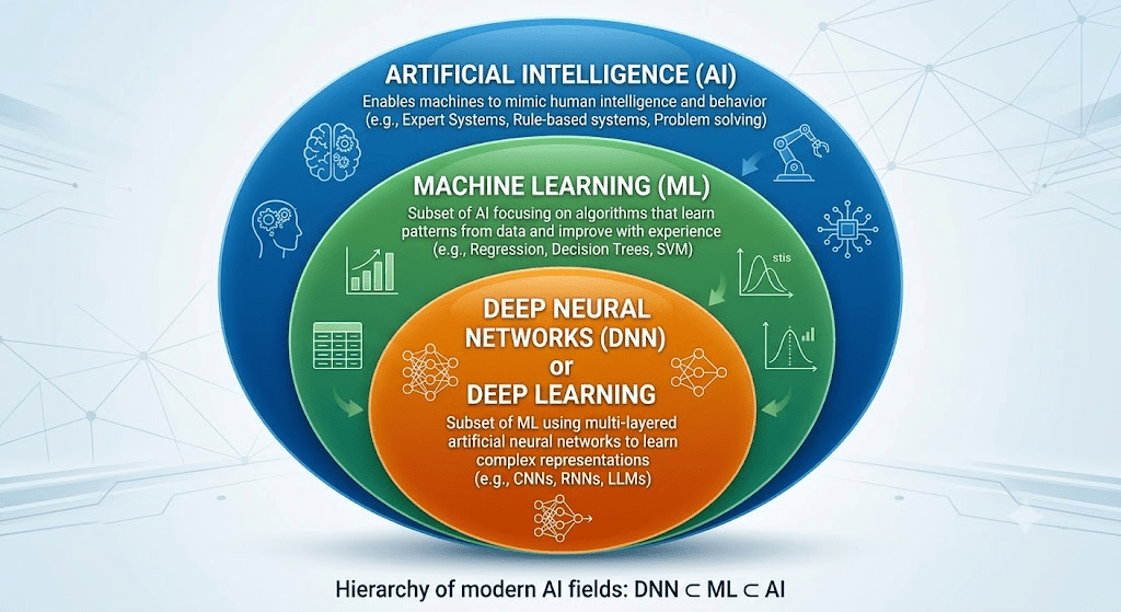
Diagram – Hierarchy : AI , ML , DNN

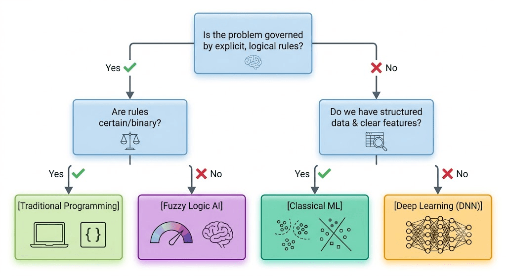
  1. Traditional programming – Crisp logic – You write an if/else statement defining anything >30 °C as Hot. Crisp logic is a Traditional programming logic . No data needed.
  2. AI is Rule driven which involves fuzzy logic (a human expert must still sit down and write every single rule ).No data needed.
  3. ML is data driven – then ML is helpful and data is requried.
  4. when we don’t have exact features then comes powerful DNN.

When to use which:


Types Of ML

Based on level of supervision:

  1. Supervised
    1. Regression – numerical
    2. Classification
  2. Unsupervised
    1. Clustering
    2. Anomaly
    3. Association
  3. Semi supervised
  4. Reinforcement
    • reward/punishment mechanism

Based on mode of training:

  1. Batch/offline
    • Offline learning of ML system
    • When to use? no concept drift e.g. Classification
      • cons – heavy size
  2. Online
    • learning in small sizes – chuck of data – can be done on production environment.
    • When to use?
      • Concept drift e,g. stock market etc.
      • Faster solution

Based on learning

  • Instance based
    • the system learns the training examples by heart. When a new data point arrives, it doesn’t look at a formula; it looks back at its memorized data and compares the new point to its closest neighbors.
      • example –
        • K-Nearest Neighbors (KNN). If you want to predict if a customer will default on a loan, KNN looks at the K closest customers in its database who have similar income/age and takes a majority vote.
        • SVM – Support vector machine
  • Model based
    • the algorithm takes the training data, uncovers the underlying pattern, and condenses that pattern into a fixed mathematical formula (a model). Once the formula is created, the original data can be thrown away.
      • Example- Linear Regression (y = mx + c) or Logistic Regression. Once the model learns the exact values for m and c, it deletes the training data from its memory. To predict y for a new x, it just runs that basic equation.

Challenges in ML

  1. Data collection
  2. Insufficient data/labelled data
  3. Non representative data
    • Sampling Noise
      • Sampling Noise (often called sampling error or variance) is the purely random fluctuation that occurs because you are looking at a smaller sample instead of the entire universe of data.
    • Sampling Bias
      • Sampling Bias occurs when your sample is collected in a way that some members of the intended population are less likely or more likely to be included than others. e.g from 4 countries only view of specific nationality person are taken on – which country will win cricket world-cup.
  4. Poor quality data – 60% on time is consumed in correcting poor data – .
  5. Irrelevant features – Saying GIGO
    • Feature engineering
  6. Overfitting
  7. Underfitting
  8. Software Integration
    • Integration becomes difficult because not all libraries are natively supported in every other language which is used to run the software
  9. Offline learning & deployment
  10. Cost involved

Application of ML

  1. Product recommendation
  2. Chatbot
  3. B2B
    • Retail (e-commerce)
      • Before Sale – Predicting which skus will be most in demand
        • Has huge impact financially if correctly predicted – not unnecessary stocking, if wrongly Out of stock issue
        • Usually Companies maintain user profile based on buying interest. used in targeting marketing
        • Positioning of products – Association rule (baby diapers and beer paper)
    • Finance
      • Loan – profile is compared against past defaulters how many changes of overlapping criteria.
      • Sharemarket
    • Transportation
      • Ola/Uber – Price surge. – “Prices are higher because of increased demand“
    • Manufacturing (Tesla car)
      • Predictive maintenance – based on input before product goes off , it is repaired
    • Banking
    • Social Media(Twitter)
      • Sentiment analysis
  4. B2C

Machine Learning Development lifecycle

It has around 9 steps (Mind the sequence of 3->4->5 and onwards it comes as is):

  1. Frame the problem
  2. Data gathering
  3. Preprocessing
    • Remove duplicates
    • Remove missing values etc.
  4. EDA – Exploratory Data Analysis – EDA is how you find those patterns.
    1. univariate analysis
      • Categorical Data: You use Bar Charts or frequency counts to identify class imbalances (e.g., checking if $95\%$ of rows are “Approve” and only $5\%$ are “Reject”).
      • Numerical Data: You plot Histograms or Kernel Density Estimate (KDE) plots. You are checking for skewness (is the data normally distributed, or heavily shifted?).
    2. bivariate analysis
      • Scatter Plots: To check if two numerical variables have a linear or non-linear relationship.
    3. Outlier detection
  5. Feature selection
    • Feature combination – because more the feature more is the cost.
    • Feature scaling
  6. Model Training, Analysis and selection
    • ensemble learning – multiple algos combined to give better algo for a problem
  7. Testing
  8. Deployment
  9. Optimisation

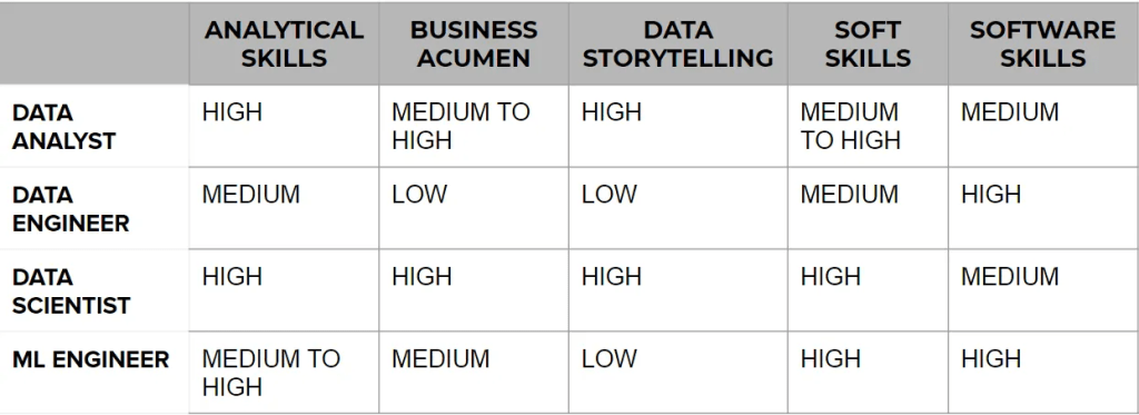
Job Roles in the field

  1. Data Engineer – Core responsibility is fetching the data from different sources and making one warehouse for OLAP
  2. Data Analyst – More like Business Analyst but involve a bit more technicality.
  3. Data Scientist – Core responsibility is how to use the data for future business- where as DA gives the historical analysis, this role is more of a Full-stack kind.
  4. Machine Learning Engineer – Core responsibility Model optimisation and training , integrating with software , Data Optimisation and deployment of Model etc.

Conclusion :

Phase 1 – Building Blocks

SubjectCore Concepts to ApplyProject/Application Use Case (E-commerce & Fintech)
Mathematical Foundations for ML (AIMLZC416)Vector algebra, Gradient descent, & PCA.ML System Optimization: Using PCA for dimensionality reduction to optimize the performance of the ClickHouse-powered analytics dashboard you built at xyz.
Introduction to Statistical Methods (AIMLZC418)Bayes Theorem, Hypothesis Testing, & Time series analysis.Inventory Forecasting: Applying ARIMA/SARIMA time series models to your SKU-level inventory API at abc to predict stock-outs with higher statistical significance.
Machine Learning (AIMLZG565)Supervised/Unsupervised Learning & Ensemble methodsIntelligent Fraud Detection: Utilizing Random Forest or SVMs to enhance the real-time reconciliation system designed for upi payments at xyz.
Deep Neural Networks (AIMLZG511)Backpropagation, CNNs, & Transformers.B2B Communication Intelligence: Using Transformer-based NLP models to extract intent and automate tracking from the Order Notes API you designed.