Graph

Index

  1. Introduction
  2. Dijkstra Algorithm
  3. Bellman-ford Algorithm
  4. Floyd-Warshall Algorithm
  5. Prim’s Algorithm

Introduction

Common Terminology –

  1. Minimum Spanning Tree (MST) used in prims algorithm
    • Goal: To connect all vertices in a graph with the minimum possible total edge weight, without forming any cycles.
    • Output: A tree that spans all vertices of the graph with the minimum sum of edge weights.
  2. Shortest path
    • Goal: To find the shortest path between a specific pair of vertices in a graph, minimizing the sum of the edge weights along that path.
    • Output: A path (which may include some or all vertices) with the minimum possible total weight between two specific vertices.

Dijkstra Algorithm

  1. Purpose: Finds the shortest path from a single source to all other vertices in a graph.
  2. Applicability: Works only with graphs that have non-negative edge weights.
  3. Woking:
    • Uses a greedy approach.
    • Iteratively selects the vertex with the smallest known distance, explores its neighbors, and updates their distances.
    • Once a vertex is processed, its shortest path is finalised.

Dijkstra’s algorithm is like breadth-first search  (BFS), except we use a priority queue  instead of a normal first-in-first-out queue.  Each item’s priority is the cost of reaching it.

Note-Implementation is similar to Prim’s algorithm for minimum spanning tree.


REf-

  1. https://www.interviewcake.com/concept/java/dijkstras-algorithm (desciption working in chart)
  2. https://www.tutorialcup.com/interview/algorithm/dijkstra-algorithm.htm (application + short implemntation)
  3. https://www.interviewbit.com/tutorial/dijkstra-algorithm/ (Pseudo code + Graph Algo)
    1. https://www.interviewbit.com/tutorial/breadth-first-search/#breadth-first-search

Bellman-Ford Algorithm


  1. Purpose: Also finds the shortest path from a single source to all other vertices, but can handle graphs with negative edge weights.
  2. Applicability: Works with graphs that may have negative edge weights, and can also detect negative weight cycles (where a cycle’s total weight is negative).
  3. Woking:
    • Uses a dynamic programming approach.
    • Iteratively relaxes all edges, meaning it updates the shortest path estimate for each edge based on its current known distance.
    • After V−1V-1V−1 iterations, it ensures that the shortest paths are found. If an additional relaxation improves any distance, it indicates a negative weight cycle.


Floyd-Warshall Algorithm

  1. Purpose: Finds the shortest paths between all pairs of vertices in a graph.
  2. Applicability: Works with both directed and undirected graphs, including those with negative edge weights.
  3. Wokings:
    • Uses a dynamic programming approach.
    • Iteratively updates a distance matrix where each entry dist[i][j] represents the shortest path from vertex i to vertex j.
    • Considers each vertex as an intermediate point in the path and updates the matrix accordingly.


Prim’s Algorithm

  1. Purpose: Finds the Minimum Spanning Tree (MST) of a connected, undirected graph. The MST is a subset of the edges that connects all vertices together, without any cycles, and with the minimum possible total edge weight.
  2. Applicability: Works with weighted, undirected graphs. It requires that the graph be connected, meaning there must be a path between every pair of vertices.
Arrays Algorithms

  1. Boyer-Moore Majority Voting Algorithm
  2. Kadane’s Algo

Boyer-Moore Majority Voting Algorithm

A majority element is one that appears more than nums.length / 2 times.

Algorithm Proceeding-

  1. First, choose a candidate from the given set of elements
  2. if it is the same as the candidate element, increase the votes. Otherwise,
    • decrease the votes if votes become 0, select another new element as the new candidate.
public static int findMajorityElement(int[] nums) {
        int majorityElement = 0;
        int count = 0;
        
        for (int num : nums) {
            if (count == 0) {
                majorityElement = num;
                count = 1;
            } else if (num == majorityElement) {
                count++;
            } else {
                count--;
            }
        }
}
        

Kadane’s Algo

Kadane’s algorithm a popular dynamic programming algorithm, it is used for finding the maximum sum of a contiguous subarray in an array. it efficiently handles both positive and negative numbers.

Conditions/Cases to remember

  • does it handle empty array?[NA]
  • does it handle all -ve element, i.e what will be the ans in this case, since sum of 2 -ve is grater -ve number. [YES]
  • should we consider using 0 or arr[i] as substitution in code – Any works ,but corresponding initiation & iteration required.

It works by maintaining two variables:maxSoFar & maxEndingHere

  1. maxSoFar stores the maximum sum of any contiguous subarray seen so far, and
  2. maxEndingHere stores the maximum sum of any contiguous subarray ending at the current index.
public static int maxSubArraySum(int[] nums) {
int maxSoFar=Integer.MIN_VALUE;//final result initiated to min not 0, for cases where elements with -ve numbers would result in max being 0 -which is incorrect.
        int maxEndingHere=0;
        for(int i=0;i<nums.length;i++){
            maxEndingHere=Math.max(nums[i]+maxEndingHere,nums[i]);
            maxSoFar=Math.max(maxSoFar,maxEndingHere);
        }
      return maxSoFar;  
}

Sorting Algorithms

Index

  1. Time Complexities
  2. Selection sort
  3. Bubble sort
  4. Insertion sort
  5. Quick Sort sort
  6. Merge Sort sort
  7. Heap sort

Time-Complexity of Sorting-Algorithms

ALGORITHMWORST-case Time Complexity(Big O Notation)AVERAGE-case time complexity (Theta Notation)BEST-case time-complexity (Omega Notation)
Selection sortingO(n^2)θ(n^2)Ω(n^2)
Bubble sortingO(n^2)θ(n^2)Ω(n)
Insertion sortingO(n^2)θ(n^2)Ω(n)
Heap sortingO(nlog(n))θΩ
Quick sortingO(n^2)θΩ
Merge sortingO(nlog(n))θΩ
Bucket sortingO(n^2)θΩ
Radix sortingO(nk)θΩ
Tree-sort O(nlog(n))

Working of Sorting Algorithms


Usage : Selection vs Insertion vs Bubble sort

  1. Selection Sort is best when memory write operations are costly since it makes the minimum possible number of swaps compared to other two.
  2. Insertion Sort is preferable for small or nearly sorted data.
  3. Bubble Sort is typically used for educational purposes to demonstrate sorting techniques but is rarely used in practical applications due to its inefficiency.

Selection Sorting


Algorithm :

  1. Iterate through the array to find the smallest (or largest) element.
  2. Swap the found minimum (or maximum) element with the first element.
  3. Move the boundary of the unsorted subarray by one element.
  4. Repeat the process for the remaining unsorted portion of the array.

  private static void selectionSort(int[] arr) {
        int n = arr.length;
        for (int i = 0; i < n; i++) {
            int minIndex = i;
            for (int j = i + 1; j < n; j++) {
                if (arr[j] < arr[minIndex]) {
                    minIndex = j;
                }
            }
//optimisation used :  outer loop used for swapping - internal for index tracking
            int temp = arr[minIndex];
            arr[minIndex] = arr[i];
            arr[i] = temp;

        }
    }
  1. Time Complexity: O(n²)
  2. Space Complexity: O(1) (In-place sorting)

Bubble Sort

Algorithm :

  1. Compare adjacent elements in the array.
  2. Swap them if they are in the wrong order.
  3. Continue doing this for each pair of adjacent elements until the array is fully sorted
  4. .After each pass, the next largest element is in its correct position.
  5. Repeat the process until no swaps are needed (the array is sorted).

  private static void bubbleSort(int[] arr) {
        int n = arr.length;
        for (int i = 0; i < n - 1; i++) {

            for (int j = 0; j < n - 1; j++) {
                if(arr[j]>arr[j+1]){
                    int temp=arr[j+1];
                    arr[j+1]=arr[j];
                    arr[j]=temp;
                }
            }
        }
     
    }
  1. Time Complexity: O(n²)
  2. Space Complexity: O(1) (In-place sorting)

Insertion Sort

Algorithm :

  1. Start from the second element, assume that the first element is already sorted.
  2. Pick the next element and compare it with the elements in the sorted part.
  3. Shift all elements in the sorted part that are greater than the current element to the right.
  4. Insert the current element into its correct position.
  5. Repeat the process until the entire array is sorted.

 public static void insertionSort(int[] arr) {
        int n = arr.length;
        for (int i = 1; i < n; i++) {
            int key = arr[i];
            int j = i - 1;
            // Move elements of arr[0..i-1] that are greater than key to one position ahead
            while (j >= 0 && arr[j] > key) {
                arr[j + 1] = arr[j];
                j = j - 1;
            }
            arr[j + 1] = key;
        }
    }
  1. Time Complexity: O(n²)
  2. Space Complexity: O(1) (In-place sorting)

Quick Sort

Algorithm :

  1. Choose a “pivot” element from the array.
  2. Partition the array into two sub-arrays: elements less than the pivot and elements greater than the pivot.
  3. Recursively apply the same steps to the sub-arrays.
  4. Combine the sub-arrays to get the sorted array.
  public static void quickSort(int[] arr, int low, int high) {
        if (low < high) {
            int pi = partition(arr, low, high);
            quickSort(arr, low, pi - 1);  // Recursively sort elements before partition
            quickSort(arr, pi + 1, high); // Recursively sort elements after partition
        }
    }

    private static int partition(int[] arr, int low, int high) {
        int pivot = arr[high];
        int i = (low - 1); // Index of smaller element
        for (int j = low; j < high; j++) {
            if (arr[j] < pivot) {
                i++;
                // Swap arr[i] and arr[j]
                int temp = arr[i];
                arr[i] = arr[j];
                arr[j] = temp;
            }
        }
        // Swap arr[i+1] and arr[high] (or pivot)
        int temp = arr[i + 1];
        arr[i + 1] = arr[high];
        arr[high] = temp;

        return i + 1;
    }
  1. Time Complexity:
    • Best Case: O(n log n)
    • Worst Case: O(n²) (occurs when the smallest or largest element is always chosen as the pivot)
  2. Space Complexity: O(log n) (in-place sorting, though recursion stack takes

Merge Sort

Algorithm :

  1. Divide the array into two halves.
  2. Recursively sort each half.
  3. Merge the two halves to create a sorted array.
public class MergeSort {
    public static void mergeSort(int[] arr, int left, int right) {
        if (left < right) {
            int middle = (left + right) / 2;
            // Sort first and second halves
            mergeSort(arr, left, middle);
            mergeSort(arr, middle + 1, right);
            // Merge the sorted halves
            merge(arr, left, middle, right);
        }
    }

    private static void merge(int[] arr, int left, int middle, int right) {
        int n1 = middle - left + 1;
        int n2 = right - middle;

        // Temporary arrays
        int[] L = new int[n1];
        int[] R = new int[n2];

        // Copy data to temp arrays
        for (int i = 0; i < n1; i++)
            L[i] = arr[left + i];
        for (int j = 0; j < n2; j++)
            R[j] = arr[middle + 1 + j];

        // Merge the temp arrays
        int i = 0, j = 0;
        int k = left;
        while (i < n1 && j < n2) {
            if (L[i] <= R[j]) {
                arr[k] = L[i];
                i++;
            } else {
                arr[k] = R[j];
                j++;
            }
            k++;
        }

        // Copy remaining elements of L[]
        while (i < n1) {
            arr[k] = L[i];
            i++;
            k++;
        }

        // Copy remaining elements of R[]
        while (j < n2) {
            arr[k] = R[j];
            j++;
            k++;
        }
    }

    public static void main(String[] args) {
        int[] arr = {12, 11, 13, 5, 6, 7};
        
        // Call mergeSort with the full range of the array
        mergeSort(arr, 0, arr.length - 1);
        
        // Print the sorted array
        System.out.println("Sorted array:");
        for (int num : arr) {
            System.out.print(num + " ");
        }
    }
}


Heap sort


Algorithm :


Introduction

  1. Asymptotic Analysis and notation
  2. Sorting Algorithms- nlogn
    1. Insertion sort
    2. Selection sort
    3. Bubble sort
    4. Merge SOrt
    5. Quick Sort
    6. Heap sort
  3. Searching Algorithms (log(n)-tree)
    1. Linear search
    2. Binary search
    3. DFS
    4. BFS
  4. Arrays
    1. Boyer-Moore Majority Voting Algorithm
    2. Kadane’s Algo
    3. Floyd’s cycle detection
    4. KMP
    5. Quick select
  5. Graph
    1. Dijkstra Algorithm
    2. Kruskal Algo
    3. Bellman ford Algo
    4. floyd warshall Algo
    5. topological sort Algo
    6. Flood fill Algo
    7. lee Algo
  6. Basic Algos
    1. Euclids Algo
    2. Union Find Algo
    3. Huffman coding compression Algo
S.No.AlgorithmAlgorithm Design paradigm
1Dijkstra shortest pathBFS
2Floyd-Warshall algorithm – to compute all-pairs shortest pathGreedy design
3Binary search on sorted arrayDynamic programming
4Backtracking search on graphDivide and conquer
5DFS
Match the correct once

Scala

Topics to be covered

  1. Introduction
    1. Why Scala?
    2. Frameworks
    3. Java Vs Scala
    4. Installation
    5. Versions
  2. Functional Programming Concepts
    1. Immutability
    2. Expressions vs statements
    3. Functions
    4. Pure and impure functions
    5. refrential transperency
    6. Higher order function
  3. First Interaction with scala
    1. repl
    2. variable and values
    3. condtionals
    4. loops
  4. Functions
    1. Structure of function
    2. anonymous function
    3. Higher order function
  5. Collection
  6. Concurrency

References

  1. Scala The Big Picture
    1. Plural Sight – Harit Himanshu

Low Level Design

Index:

  1. Introduction & Representation techniques
    1. OOAD (Object Oriented Analysis and Design) – CDAC reference
      1. Representation using UML(Unified Modelling Language) notation
      2. For Drawing UML Tools-
        • Offline- StarUML,
        • Online – Diagrams.net
      3. OO Analysis and Design Methodolgy
      4. OO Notation
      5. OO tool to draw OOAD Design
  2. OOP (implementation)
    1. OOP Principal
      1. P.I.E.A.
    2. SOLID
    3. Association, Aggregation, Composition
  3. Design pattern (implementation)
    • Behavioural
    • Creational
    • Structural
  4. Interview Outline

What does a OO Designer needs?

  1. OO Concepts
  2. OO Language
  3. OO Analysis and Design Methodolgy
  4. OO Notation
  5. OO tool to draw OOAD Design

OOAD Techniques

  1. Fusion
  2. Jacobson
  3. Rumbaugh
  4. Booch
  5. Rational Unified Process (RUP) with Unified Modeling Language (UML)

OO Design Tools

  1. Rational Software
  2. StarUML

UML Diagrams for OOAD design using RUP

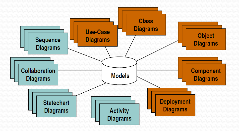
At core we have Models and using which various representation can be drawn for specific analysis-

  1. Use-case Diagrams
  2. Class Diagrams
  3. Object Diagrams
  4. State-chart Diagrams
  5. Sequence Diagrams

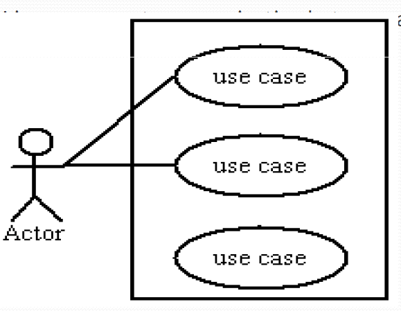
Use Case Analysis – Drawing the Use Case Diagram

My take- useful in case of establishing relation between use-case/functionality

  • Stick Figure Represents Actor
  • Oval Represents Use Case
  • The Rectangle represents System Boundary

Use Case Analysis – Use Case Relationships

3 kinds of relationships between use cases

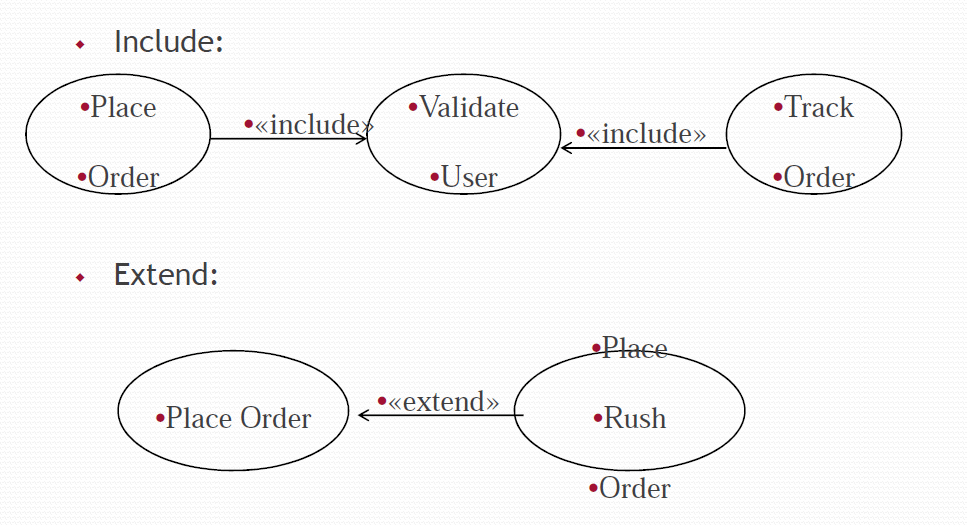
  1. Include
  2. Extend
  3. Uses

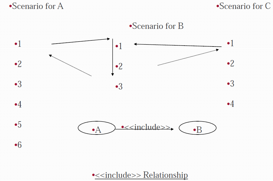
Include:

  1. «include» stereotype indicates that one use case “includes” the contents of another use case.
  2. Enables factoring out frequent common behavior

Use case “A” includes use case “B” if :

  1. B describes scenario which is part of scenario of A &
  2. B describes scenario common for a set of use cases including A

Extends:

  1. «extend» stereotype indicates that one use case is “extended” by another use case.
  2. Enables factoring out infrequent behavior or error conditions
  3. Used to show optional behaviour for a use case which will be required only under certain conditions

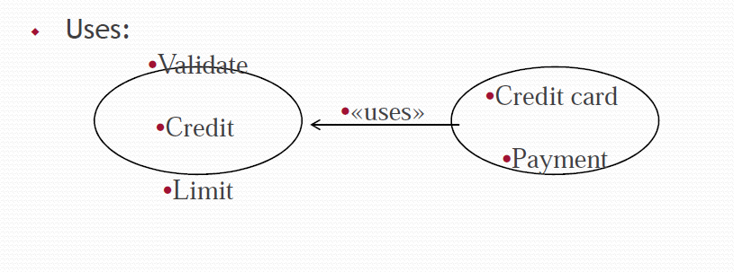
Uses:

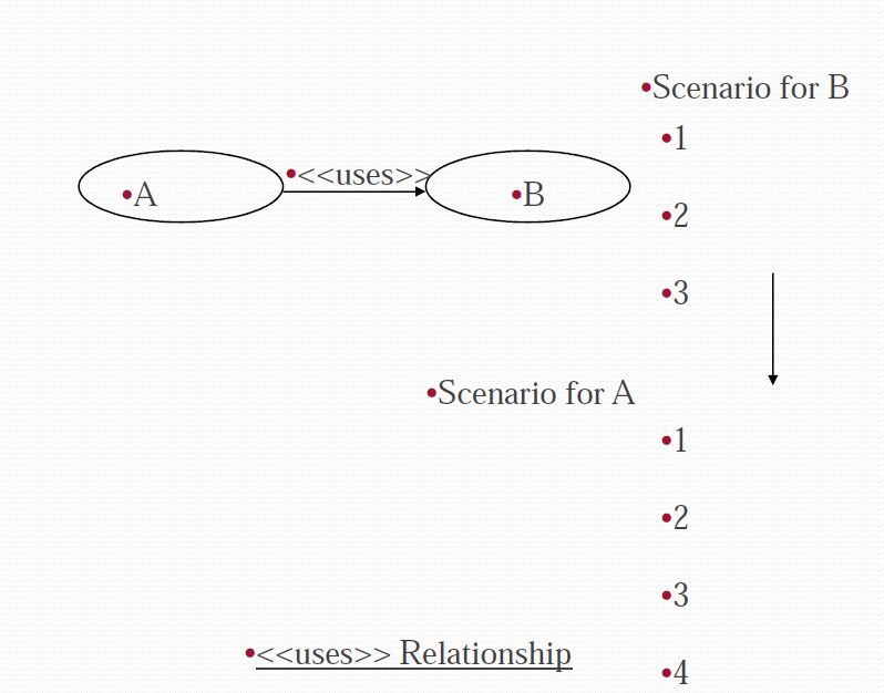
  1. «uses» stereotype indicates that one use case is precondition for executing another use case
  2. Use case “A” uses use case “B” if
    1. B describes a scenario which is not part of scenarios carrying out service A &
    2. B is a precondition for successful invocation of A

Examples


OOAD: Activity Diagram

Depicts business processes and data flows to model the complex logic within the system


OOAD: Sequence Diagrams

Models the time ordering of messages between classifiers to accomplish given
functionality


UML Diagrams: Collaboration Diagrams

Focuses on the structural organisation of objects that send and receive messages.
Known as communication diagrams in UML 2.0.


UML Diagrams: Class Diagrams

Models a collection of static model elements such as classes, their contents and
relationships


UML Diagrams: State machine Diagrams

Describes states of an object and transitions between the states


UML Diagrams: Component Diagrams

Depicts the components, their interfaces and interrelationships


UML Diagrams: Deployment Diagrams

Shows the execution architecture of the application

Dynamic Programming

Index

  1. Introduction to Dynamic Programming
    1. Strategic Approach
    2. Common patterns
      • Top-Down Approach – recursion+memorisation
      • Bottom-up Approach – tabulation.

Introduction to Dynamic Programming

What is Dynamic Programming?

Dynamic Programming (DP) is a programming paradigm that can systematically and efficiently explore all possible solutions to a problem. As such, it is capable of solving a wide variety of problems that often have the following characteristics:

  1. The problem can be broken down into “overlapping subproblems” – smaller versions of the original problem that are re-used multiple times.
  2. The problem has an “optimal substructure” – an optimal solution can be formed from optimal solutions to the overlapping subproblems of the original problem.

Fibonacci Example –

If you wanted to find the n^{th}nth Fibonacci number F(n)F(n), you can break it down into smaller subproblems – find F(n – 1)F(n−1) and F(n – 2)F(n−2) instead. Then, adding the solutions to these subproblems together gives the answer to the original question, F(n – 1) + F(n – 2) = F(n)F(n−1)+F(n−2)=F(n), which means the problem has optimal substructure, since a solution F(n)F(n) to the original problem can be formed from the solutions to the subproblems. These subproblems are also overlapping – for example, we would need F(4)F(4) to calculate both F(5)F(5) and F(6)F(6).

These attributes may seem familiar to you. Greedy problems have optimal substructure, but not overlapping subproblems. Divide and conquer algorithms break a problem into subproblems, but these subproblems are not overlapping (which is why DP and divide and conquer are commonly mistaken for one another).

There are two ways to implement a DP algorithm:

  1. Bottom-up, also known as tabulation.
  2. Top-down, also known as memoization.

Bottom-up (Tabulation)

Bottom-up is implemented with iteration and starts at the base cases. Let’s use the Fibonacci sequence as an example again. The base cases for the Fibonacci sequence are F(0)=0 and F(1) = 1. With bottom-up, we would use these base cases to calculate F(2)F(2), and then use that result to calculate F(3), and so on all the way up to F(n)

Pseudi COde

// Pseudocode example for bottom-up

F = array of length (n + 1)
F[0] = 0
F[1] = 1
for i from 2 to n:
    F[i] = F[i - 1] + F[i - 2]

Top-down (Memoization)

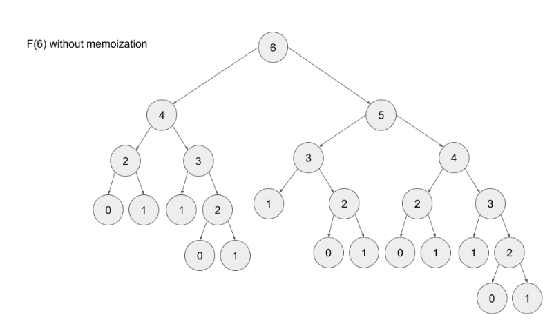
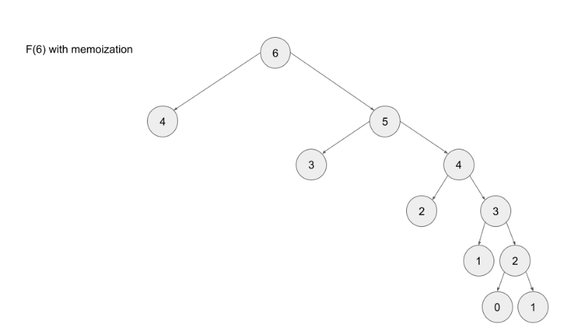
Top-down is implemented with recursion and made efficient with memoization. If we wanted to find the n^{th}nth Fibonacci number F(n)F(n), we try to compute this by finding F(n – 1)F(n−1) and F(n – 2)F(n−2). This defines a recursive pattern that will continue on until we reach the base cases F(0) = F(1) = 1F(0)=F(1)=1. The problem with just implementing it recursively is that there is a ton of unnecessary repeated computation. Take a look at the recursion tree if we were to find F(5)F(5):

Notice that we need to calculate F(2) three times. This might not seem like a big deal, but if we were to calculate F(6), this entire image would be only one child of the root. Imagine if we wanted to find F(100) – the amount of computation is exponential and will quickly explode. The solution to this is to memoize results.

Note- memoizing a result means to store the result of a function call, usually in a hashmap or an array, so that when the same function call is made again, we can simply return the memoized result instead of recalculating the result.

Advantages

  • It is very easy to understand and implement.
  • It solves the subproblems only when it is required.
  • It is easy to debug.

Disadvantages

  • It uses the recursion technique that occupies more memory in the call stack.
  • Sometimes when the recursion is too deep, the stack overflow condition will occur.
  • It occupies more memory that degrades the overall performance.

When to Use DP

Following are the scenarios to use DP-

  1. The problem can be broken down into “overlapping subproblems” – smaller versions of the original problem that are re-used multiple times
  2. The problem has an “optimal substructure” – an optimal solution can be formed from optimal solutions to the overlapping subproblems of the original problem.

Unfortunately, it is hard to identify when a problem fits into these definitions. Instead, let’s discuss some common characteristics of DP problems that are easy to identify.

The first characteristic that is common in DP problems is that the problem will ask for the optimum value (maximum or minimum) of something, or the number of ways there are to do something. For example:

  • Optimization problems.
    • What is the minimum cost of doing…
    • What is the maximum profit from…
    • How many ways are there to do…
    • What is the longest possible…
    • Is it possible to reach a certain point…
  • Combinatorial problems.
    • given a number N, you’ve to find the number of different ways to write it as the sum of 1, 3 and 4.

Note: Not all DP problems follow this format, and not all problems that follow these formats should be solved using DP. However, these formats are very common for DP problems and are generally a hint that you should consider using dynamic programming.

When it comes to identifying if a problem should be solved with DP, this first characteristic is not sufficient. Sometimes, a problem in this format (asking for the max/min/longest etc.) is meant to be solved with a greedy algorithm. The next characteristic will help us determine whether a problem should be solved using a greedy algorithm or dynamic programming.

The second characteristic that is common in DP problems is that future “decisions” depend on earlier decisions. Deciding to do something at one step may affect the ability to do something in a later step. This characteristic is what makes a greedy algorithm invalid for a DP problem – we need to factor in results from previous decisions.

Algorithm –

You can either use Map or array to store/memoize the elements (both gives O(1) access time.